16 Web scraping

The data we need to answer a question is not always in a spreadsheet ready for us to read. For example, the US murders dataset we used in the R Basics chapter originally comes from this Wikipedia page:

url <- paste0("https://en.wikipedia.org/w/index.php?title=",
              "Gun_violence_in_the_United_States_by_state",
              "&direction=prev&oldid=810166167")

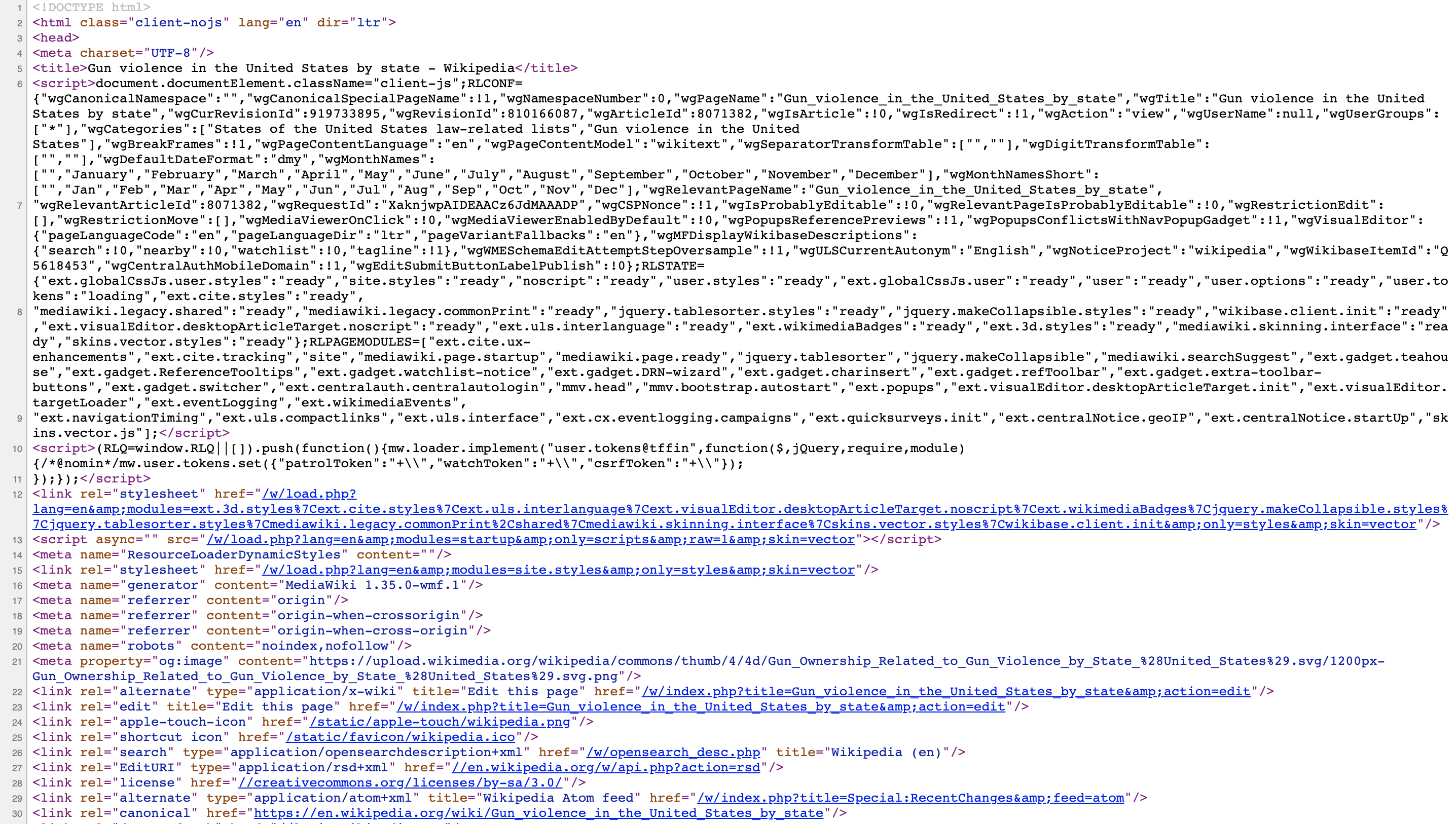
You can see the data table when you visit the webpage:

(Web page courtesy of Wikipedia¹. CC-BY-SA-3.0 license². Screenshot of part of the page.)

Web scraping, or web harvesting, is the term we use to describe the process of extracting data from a website. The reason we can do this is because the information used by a browser to render webpages is received as a text file from a server. The text is code written in hyper text markup language (HTML). Every browser has a way to show the html source code for a page, each one different. On Chrome, you can use Control-U on a PC and command+alt+U on a Mac. You will see something like this:

16.1 HTML

Because this code is accessible, we can download the HTML file, import it into R, and then write programs to extract the information we need from the page. However, once we look at HTML code, this might seem like a daunting task. But we will show you some convenient tools to facilitate the process. To get an idea of how it works, here are a few lines of code from the Wikipedia page that provides the US murders data:

<table class="wikitable sortable">
<tr>
<th>State</th>
<th><a href="/wiki/List_of_U.S._states_and_territories_by_population" 
title="List of U.S. states and territories by population">Population</a><br />
<small>(total inhabitants)</small><br />
<small>(2015)</small> <sup id="cite_ref-1" class="reference">
<a href="#cite_note-1">[1]</a></sup></th>
<th>Murders and Nonnegligent
<p>Manslaughter<br />
<small>(total deaths)</small><br />
<small>(2015)</small> <sup id="cite_ref-2" class="reference">
<a href="#cite_note-2">[2]</a></sup></p>
</th>
<th>Murder and Nonnegligent
<p>Manslaughter Rate<br />
<small>(per 100,000 inhabitants)</small><br />
<small>(2015)</small></p>
</th>
</tr>
<tr>
<td><a href="/wiki/Alabama" title="Alabama">Alabama</a></td>
<td>4,853,875</td>
<td>348</td>
<td>7.2</td>
</tr>
<tr>
<td><a href="/wiki/Alaska" title="Alaska">Alaska</a></td>
<td>737,709</td>
<td>59</td>
<td>8.0</td>
</tr>
<tr>

You can actually see the data, except data values are surrounded by html code such as <td>. We can also see a pattern of how it is stored. If you know HTML, you can write programs that leverage knowledge of these patterns to extract what we want. We also take advantage of a language widely used to make webpages look “pretty” called Cascading Style Sheets (CSS). We say more about this in Section 16.3.

Although we provide tools that make it possible to scrape data without knowing HTML, it is useful to learn some HTML and CSS. Not only does this improve your scraping skills, but it might come in handy if you are creating a webpage to showcase your work. There are plenty of online courses and tutorials for learning these. Two examples are Codeacademy³ and W3schools⁴.

16.2 The rvest package

The tidyverse provides a web harvesting package called rvest. The first step using this package is to import the webpage into R. The package makes this quite simple:

library(tidyverse)
library(rvest)
h <- read_html(url)

Note that the entire Murders in the US Wikipedia webpage is now contained in h. The class of this object is:

class(h)
#> [1] "xml_document" "xml_node"

The rvest package is actually more general; it handles XML documents. XML is a general markup language (that’s what the ML stands for) that can be used to represent any kind of data. HTML is a specific type of XML specifically developed for representing webpages. Here we focus on HTML documents.

Now, how do we extract the table from the object h? If you were to print h, we would see information about the object that is not very informative. We can see all the code that defines the downloaded webpage using the html_text function like this:

html_text(h)

We don’t show the output here because it includes thousands of characters. But if we look at it, we can see the data we are after are stored in an HTML table: you can see this in this line of the HTML code above <table class="wikitable sortable">. The different parts of an HTML document, often defined with a message in between < and > are referred to as nodes. The rvest package includes functions to extract nodes of an HTML document: html_nodes extracts all nodes of different types and html_node extracts the first one. To extract the tables from the html code we use:

tab <- h |> html_nodes("table")

Now, instead of the entire webpage, we just have the html code for the tables in the page:

tab
#> {xml_nodeset (2)}
#> [1] <table class="wikitable sortable"><tbody>\n<tr>\n<th>State\n</th> ...
#> [2] <table class="nowraplinks hlist mw-collapsible mw-collapsed navbo ...

The table we are interested is the first one:

tab[[1]]
#> {html_node}
#> <table class="wikitable sortable">
#> [1] <tbody>\n<tr>\n<th>State\n</th>\n<th>\n<a href="/wiki/List_of_U.S ...

This is clearly not a tidy dataset, not even a data frame. In the code above, you can definitely see a pattern and writing code to extract just the data is very doable. In fact, rvest includes a function just for converting HTML tables into data frames:

tab <- tab[[1]] |> html_table()
class(tab)
#> [1] "tbl_df"     "tbl"        "data.frame"

We are now much closer to having a usable data table:

tab <- tab |> setNames(c("state", "population", "total", "murder_rate")) 
head(tab)
#> # A tibble: 6 × 4
#>   state      population total murder_rate
#>   <chr>      <chr>      <chr>       <dbl>
#> 1 Alabama    4,853,875  348           7.2
#> 2 Alaska     737,709    59            8  
#> 3 Arizona    6,817,565  309           4.5
#> 4 Arkansas   2,977,853  181           6.1
#> 5 California 38,993,940 1,861         4.8
#> # ℹ 1 more row

We still have some wrangling to do. For example, we need to remove the commas and turn characters into numbers. Before continuing with this, we will learn a more general approach to extracting information from web sites.

16.3 CSS selectors

The default look of a webpage made with the most basic HTML is quite unattractive. The aesthetically pleasing pages we see today are made using CSS to define the look and style of webpages. The fact that all pages for a company have the same style usually results from their use of the same CSS file to define the style. The general way these CSS files work is by defining how each of the elements of a webpage will look. The title, headings, itemized lists, tables, and links, for example, each receive their own style including font, color, size, and distance from the margin. CSS does this by leveraging patterns used to define these elements, referred to as selectors. An example of such a pattern, which we used above, is table, but there are many, many more.

If we want to grab data from a webpage and we happen to know a selector that is unique to the part of the page containing this data, we can use the html_nodes function. However, knowing which selector can be quite complicated. In fact, the complexity of webpages has been increasing as they become more sophisticated. For some of the more advanced ones, it seems almost impossible to find the nodes that define a particular piece of data. However, selector gadgets actually make this possible.

SelectorGadget⁵ is piece of software that allows you to interactively determine what CSS selector you need to extract specific components from the webpage. If you plan on scraping data other than tables from html pages, we highly recommend you install it. A Chrome extension is available which permits you to turn on the gadget and then, as you click through the page, it highlights parts and shows you the selector you need to extract these parts. There are various demos of how to do this including rvest author Hadley Wickham’s vignette⁶ and other tutorials based on the vignette⁷.

16.4 JSON

Sharing data on the internet has become more and more common. Unfortunately, providers use different formats, which makes it harder for data analysts to wrangle data into R. Yet there are some standards that are also becoming more common. Currently, a format that is widely being adopted is the JavaScript Object Notation or JSON. Because this format is very general, it is nothing like a spreadsheet. This JSON file looks more like the code you use to define a list. Here is an example of information stored in a JSON format:

#> [
#>   {
#>     "name": "Miguel",
#>     "student_id": 1,
#>     "exam_1": 85,
#>     "exam_2": 86
#>   },
#>   {
#>     "name": "Sofia",
#>     "student_id": 2,
#>     "exam_1": 94,
#>     "exam_2": 93
#>   },
#>   {
#>     "name": "Aya",
#>     "student_id": 3,
#>     "exam_1": 87,
#>     "exam_2": 88
#>   },
#>   {
#>     "name": "Cheng",
#>     "student_id": 4,
#>     "exam_1": 90,
#>     "exam_2": 91
#>   }
#> ]

The file above actually represents a data frame. To read it, we can use the function fromJSON from the jsonlite package. Note that JSON files are often made available via the internet. Several organizations provide a JSON API or a web service that you can connect directly to and obtain data. Here is an example providing information Nobel prize winners:

library(jsonlite)
nobel <- fromJSON("http://api.nobelprize.org/v1/prize.json")

This downloads a list. The first argument, named “prizes” is a table with information about Nobel prize winners. Each row holds corresponds to a particular year and category. The “laureates” column holds a list with a data frame for each winner with columns for id, firstname, surname, and motivation.

nobel$prizes |>
  filter(category == "literature" & year == "1971") |> 
  pull(laureates) |>
  first() |>
  select(id, firstname, surname)
#>    id firstname surname
#> 1 645     Pablo  Neruda

You can learn much more by examining tutorials and help files from the jsonlite package. This package is intended for relatively simple tasks such as converting data into tables. For more flexibility, we recommend the rjson package.

16.5 Data APIs

An Application Programming Interface (API) is a set of rules and protocols that allows different software entities to communicate with each other. It defines methods and data formats that software components should use when requesting and exchanging information. APIs play a crucial role in enabling the integration that make today’s software so interconnected and versatile.

There are several types of APIs. The main ones related to retrieving data are:

Web Services - Often built using protocols like HTTP/HTTPS. Commonly used to enable applications to communicate with each other over the web. For instance, a weather application for a smartphone may use a web API to request weather data from a remote server.
Database APIs - Enable communication between an application and a database, SQL-based calls for example.

Key concepts associated with APIs:

Endpoints: Specific functions available through the API. For web APIs, an endpoint is usually a specific URL where the API can be accessed.
Methods: Actions that can be performed. In web APIs, these often correspond to HTTP methods like GET, POST, PUT, or DELETE.
Requests and Responses: The act of asking the API to perform its function is a request. The data it returns is the response.
Rate Limits: Restrictions on how often you can call the API, often used to prevent abuse or overloading of the service.
Authentication and Authorization: Mechanisms to ensure that only approved users or applications can use the API. Common methods include API keys, OAuth, or Jason Web Tokens (JWT).
Data Formats: Many web APIs exchange data in a specific format, often JSON or CSV.

16.6 The httr2 package

HTTP is the most widely used protocol for data sharing through the internet. The httr2 package provides functions to work with HTTP requests. One of the core functions in this package is request, which is used to form request to send to web services. The req_perform function sends the request.

This request function forms an HTTP GET request to the specified URL. Typically, HTTP GET requests are used to retrieve information from a server based on the provided URL.

The function returns an object of class response. This object contains all the details of the server’s response, including status code, headers, and content. You can then use other httr2 functions to extract or interpret information from this response.

Let’s say you want to retrieve COVID-19 deaths by state from the CDC. By visiting their data catalog⁸ you can search for datasets and find that the data is provided through this API:

url <- "https://data.cdc.gov/resource/muzy-jte6.csv"

We can then make create and perform a request like this:

library(httr2)
response <- request(url) |> req_perform()

We can see the results of the request by looking at the returned object.

response
#> <httr2_response>
#> GET https://data.cdc.gov/resource/muzy-jte6.csv
#> Status: 200 OK
#> Content-Type: text/csv
#> Body: In memory (210808 bytes)

To extract the body, which is where the data are, we can use resp_body_string and send the result, a comma delimited string, to read_csv

library(readr)
tab <- response |> resp_body_string() |> read_csv()

We note that the returned object is only 1000 entries. API often limit how much you can download. The documentation for this API⁹ explains that we can change this limit through the $limit parameters. We can use the req_url_path_append to add this to our request:

response <- request(url) |> 
  req_url_path_append("?$limit=100000") |> 
  req_perform()

The CDC service returns data in csv format but a more common format used by web services is JSON. The CDC also provides data in json format through a the url:

url <- "https://data.cdc.gov/resource/muzy-jte6.json"

To extract the data table we use the fromJSON function from the jsonlite package.

tab <- request(url) |> 
   req_perform() |> 
   resp_body_string() |> 
   fromJSON(flatten = TRUE)

When working with APIs, it’s essential to check the API’s documentation for rate limits, required headers, or authentication methods. The httr2 package provides tools to handle these requirements, such as setting headers or authentication parameters.

16.7 Exercises

1. Visit the following web page: https://web.archive.org/web/20181024132313/http://www.stevetheump.com/Payrolls.htm

Notice there are several tables. Say we are interested in comparing the payrolls of teams across the years. The next few exercises take us through the steps needed to do this.

Start by applying what you learned to read in the website into an object called h.

2. Note that, although not very useful, we can actually see the content of the page by typing:

html_text(h)

The next step is to extract the tables. For this, we can use the html_nodes function. We learned that tables in html are associated with the table node. Use the html_nodes function to extract all tables. Store it in an object nodes.

3. The html_nodes function returns a list of objects of class xml_node. We can see the content of each one using, for example, the html_text function. You can see the content for an arbitrarily picked component like this:

html_text(nodes[[8]])

If the content of this object is an html table, we can use the html_table function to convert it to a data frame. Use the html_table function to convert the 8th entry of nodes into a table.

4. Repeat the above for the first 4 components of nodes. Which of the following are payroll tables:

All of them.
1
2
2-4

5. Repeat the above for the first last 3 components of nodes. Which of the following is true:

The last entry in nodes shows the average across all teams through time, not payroll per team.
All three are payroll per team tables.
All three are like the first entry, not a payroll table.
All of the above.

6. We have learned that the first and last entries of nodes are not payroll tables. Redefine nodes so that these two are removed.

7. We saw in the previous analysis that the first table node is not actually a table. This happens sometimes in html because tables are used to make text look a certain way, as opposed to storing numeric values. Remove the first component and then use sapply and html_table to convert each node in nodes into a table. Note that in this case, sapply will return a list of tables. You can also use lapply to assure that a list is applied.

8. Look through the resulting tables. Are they all the same? Could we just join them with bind_rows?

9. Create two tables, call them tab_1 and tab_2 using the 10th and 19th tables in nodes.

10. Use a full_join function to combine these two tables. Before you do this you will have to fix the missing header problem. You will also need to make the names match.

11. After joining the tables, you see several NAs. This is because some teams are in one table and not the other. Use the anti_join function to get a better idea of why this is happening.

12. We see see that one of the problems is that Yankees are listed as both N.Y. Yankees and NY Yankees. In the next section, we will learn efficient approaches to fixing problems like this. Here we can do it “by hand” as follows:

tab_1 <- tab_1 |>
  mutate(Team = ifelse(Team == "N.Y. Yankees", "NY Yankees", Team))

Now join the tables and show only Oakland and the Yankees and the payroll columns.

13. Advanced: extract the titles of the movies that won Best Picture from IMDB¹⁰.