17 Treatment Effect Models
Up to now, we have worked with linear models to describe relationships between continuous variables. We motivated these models using the assumption of multivariate normality and showed how the conditional expectation takes a linear form. This covers many common applications of regression.
However, linear models are not limited to describing natural variation among continuous measurements. One of the most important uses of linear models is to quantify the effect of an intervention or treatment. This framework originated in agriculture, where researchers compared crop yields across fields that received different fertilizers or planting strategies. The outcome variable was yield, and the treatment was the fertilizer. The same mathematical ideas now form the basis for analyzing randomized controlled trials in medicine, economics, public health, education, and the social sciences. Modern A/B tests used by internet companies to evaluate website changes or product features also follow this treatment effect framework.
The key idea is that a treatment defines groups, and we use linear models to estimate the difference in outcomes across these groups. In randomized experiments, the comparison is straightforward because randomization helps ensure that the groups are comparable. In observational studies, the goal is the same, but analysts must account for differences between groups that are not due to the treatment itself. For example, if we want to estimate the effect of a diet high in fruits and vegetables on blood pressure, we must adjust for factors such as age, sex, or smoking status.
17.1 Case study: high-fat diet and mouse weight
In this chapter, we consider an experiment designed to test for the effects of a high-fat diet on mouse physiology. Mice were randomly selected and divided into two groups: one group receiving a high-fat diet, considered the treatment, while the other group served as the control and received the usual chow diet. The data is included in the dslabs package:
A boxplot shows that the high-fat diet mice are, on average, heavier.
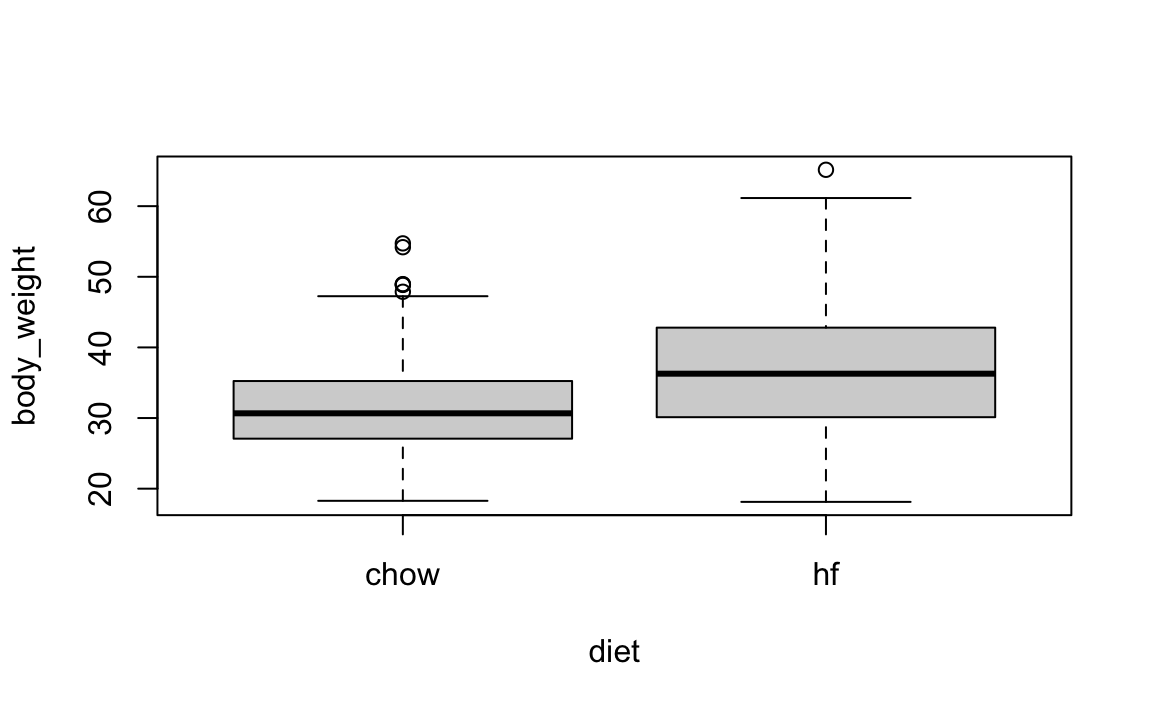
However, given that we divided the mice randomly, is it possible that the observed difference is simply due to chance?
Before making the connection to linear models, in the next section, we perform statistical inference on the difference of these means, using the approach described in Chapter 13.
17.2 Comparing group means
The sample averages for the two groups, high-fat and chow diets, are different:
We now use hypothesis testing, first described in Chapter 13, to assess whether this difference is statistically significant.
Let \(\mu_1\) and \(\sigma_1\) represent the average weight and standard deviation, respectively, that we would observe if the entire population of mice were on the high-fat diet. Define \(\mu_0\) and \(\sigma_0\) similarly, but for the chow diet. Define \(N_1\) and \(N_0\) as the sample sizes, and \(\bar{X}_1\) and \(\bar{X}_0\) the sample averages, for the high-fat and chow diets, respectively.
Since the data come from a random sample, the central limit theorem tells us that, if the sample is large enough, the distribution of the difference in averages \(\bar{X}_1 - \bar{X}_0\) can be approximated by a standard normal distribution, with expected value \(\mu_1-\mu_0\) and standard error \(\sqrt{\frac{\sigma_1^2}{N_1} + \frac{\sigma_0^2}{N_0}}\).
If we define the null hypothesis as the high-fat diet having no effect, or \(\mu_1 - \mu_0 = 0\), this implies that
\[ \frac{\bar{X}_1 - \bar{X}_0}{\sqrt{\frac{\sigma_1^2}{N_1} + \frac{\sigma_0^2}{N_0}}} \]
has expected value 0 and standard error 1 and therefore approximately follows a standard normal distribution.
Note that we can’t compute this quantity in practice because the \(\sigma_1\) and \(\sigma_0\) are unknown. However, if we estimate them with the sample standard deviations, denote them \(s_1\) and \(s_0\) for the high-fat and chow diets, respectively, the central limit theorem still holds and tells us that
\[ t = \frac{\bar{X}_1 - \bar{X}_0}{\sqrt{\frac{s_1^2}{N_1} + \frac{s_0^2}{N_0}}} \]
is approximately standard normal when the null hypothesis is true. This implies that we can easily compute the probability of observing a value as large as the one we obtained:
We can also use the R function to perform the calculation in one line:
Here \(t\) is well over 3, so we don’t really need to compute the p-value 1-pnorm(t_stat) as we know it will be very small.
Note that when \(N_0\) and \(N_1\) are not large enough, the CLT does not apply. However, as we explained in Section 10.2.3, if the outcome data, in this case weight, follows an approximately normal distribution, then the \(t\), defined above, follows a t-distribution. So the calculation of the p-value is the same except that we use pt instead of pnorm.
For the two-sample t-test used in this chapter, the appropriate degrees of freedom are not straightforward to compute when the two groups have different variances. In this setting, standard statistical texts derive an approximation based on the Welch–Satterthwaite equation.
In practice, there is no need to carry out this calculation by hand. The t.test function in R automatically uses this approximation and computes the appropriate degrees of freedom and p-value for us.
Differences in means are commonly examined in scientific studies. As a result, this t-statistic is one of the most widely reported summaries. When used to determine if an observed difference is statistically significant, we refer to the procedure as “performing a t-test”.
In the computation above, we calculated the probability of observing a \(t\) value at least as large as the one obtained. However, when our interest includes deviations in both directions–for example, either an increase or a decrease in weight–we must consider the probability of obtaining a value of \(t\) as extreme as the one observed, regardless of sign. In that case, we use the absolute value of \(t\) and double the one-sided probability: 2*(1 - pnorm(abs(t_stat)) or 2*(1-pt(abs(t_stat), with(stats, n[2]+n[1]-2))).
17.3 One-factor design
Although the t-test is useful for cases in which we compare two treatments, it is common to have other variables affect our outcomes. Linear models permit hypothesis testing in these more general situations. We start the description of the use of linear models for estimating treatment effects by demonstrating how they can be used to perform t-tests.
If we assume that the weight distributions for mice on both chow and high-fat diets are normally distributed, we can write the following linear model to represent the data:
\[ Y_i = \beta_0 + \beta_1 x_i + \varepsilon_i \]
with \(x_i = 1\) if the \(i\)-th mouse was fed the high-fat diet, and 0 otherwise, and the errors \(\varepsilon_i\) are independent and again assume a normal distribution with expected value 0 and standard deviation \(\sigma\).
Note that this mathematical formula looks exactly like the model we wrote out for the father-son heights. However, the fact that \(x_i\) is now 0 or 1 rather than a continuous variable allows us to use it in this different context. In particular, notice that now \(\beta_0\) represents the population average weight of the mice on the chow diet and \(\beta_0 + \beta_1\) represents the population average for the weight of the mice on the high-fat diet.
A nice feature of this model is that \(\beta_1\) represents the treatment effect of receiving the high-fat diet. The null hypothesis that the high-fat diet has no effect can be quantified as \(\beta_1 = 0\). We estimate \(\beta_1\) and then ask whether it is plausible for the true value to be zero.
So how do we estimate \(\beta_1\) and compute this probability? A powerful characteristic of linear models is that we can estimate the \(\beta\)s and their standard errors with the same LSE machinery:
fit <- lm(body_weight ~ diet, data = mice_weights)Because diet is a factor with two entries, the lm function knows to fit the linear model above with an \(x_i\), an indicator variable. The summary function shows us the resulting estimate, standard error, and p-value:
coefficients(summary(fit))
#>             Estimate Std. Error t value Pr(>|t|)
#> (Intercept)    31.54      0.386   81.74 0.00e+00
#> diethf          5.14      0.548    9.36 8.02e-20
If we look at the diethf row, the t value computed here is the estimate divided by its estimated standard error: \(\hat{\beta}_1 / \widehat{\mathrm{SE}}[\hat{\beta}_1]\). The Pr(>|t|) is the p-value when testing the null hypothesis that \(\beta_1=0\).
In the case of the simple one-factor model, we can show that this is almost equivalent to the t-statistics computed in the previous section, t_stat. Intuitively, it makes sense, as both \(\hat{\beta}_1\) and the numerator of the t-test are estimates of the treatment effect. The one minor difference is that the linear model does not assume a different standard deviation for each population. Instead, both populations share \(\mathrm{SD}[\varepsilon]\) as a standard deviation. Note that, although we don’t demonstrate it with R here, we can redefine the linear model to have different standard errors for each group. Also note that you can set var.equal = TRUE in the t.test function and get exactly the same result.
In the linear model description provided here, we assumed \(\varepsilon\) follows a normal distribution. This assumption permits us to show that the statistics formed by dividing estimates by their estimated standard errors follow a t-distribution, which in turn allows us to estimate p-values or confidence intervals. However, note that we do not need this assumption to compute the expected value and standard error of the least squares estimates. Furthermore, if the number of observations is large enough, then the central limit theorem applies, and we can obtain p-values and confidence intervals even without the normal distribution assumption for the errors.
17.4 Two-factor designs
We are now ready to describe a major advantage of the linear model approach over directly comparing averages.
Note that this experiment included male and female mice, and male mice are known to be heavier. This explains why the residuals depend on the sex variable:
boxplot(fit$residuals ~ mice_weights$sex)
This misspecification can have real implications; for instance, if for some reason more male mice received the high-fat diet (this should not happen with random samples), then this could explain the increase. Conversely, if fewer received it, we might underestimate the diet effect. Sex could be a confounder, indicating that our model can certainly be improved.
From examining the data:
mice_weights |> ggplot(aes(diet, log2(body_weight), fill = sex)) +
  geom_boxplot()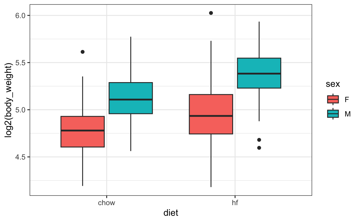
we see that the diet effect is observed for both sexes and that males are heavier than females. Although not nearly as obvious, it also appears that the diet effect is stronger in males.
A linear model that permits a different expected value for the following four groups, 1) females on the chow diet, 2) females on a high-fat diet, 3) males on the chow diet, and 4) males on a high-fat diet, can be written like this:
\[ Y_i = \beta_1 x_{i1} + \beta_2 x_{i2} + \beta_3 x_{i3} + \beta_4 x_{i4} + \varepsilon_i \]
with \(x_{i1},\dots,x_{i4}\) indicator variables for each of the four groups. With this representation, we allow the diet effect to be different for males and females.
However, in this representation, none of the \(\beta\) parameters directly correspond to the treatment effect of interest (the effect of the high-fat diet). A useful feature of linear models is that we can reparameterize the model so that the fitted means remain the same, but the coefficients have interpretations aligned with the scientific question.
For example, consider the model
\[ Y_i = \beta_0 + \beta_1 \, x_{i1} + \beta_2 \, x_{i2} + \beta_3 \,x_{i1} x_{i2} + \varepsilon_i\,, \]
where
- \(x_{i1} = 1\) if mouse \(i\) received the high-fat diet and \(0\) otherwise
- \(x_{i2} = 1\) if mouse \(i\) is male and \(0\) if female
Then we interpret the parameters as follows:
- \(\beta_0\) is the baseline average weight of females on the chow diet
- \(\beta_1\) is the diet effect for females
- \(\beta_2\) is the average difference between males and females under the chow diet
- \(\beta_3\) is the difference in the diet effect between males and females, often called an interaction effect
To see why this works, let’s examine plugging in the four options for \(x_{1i}\) and \(x_{2i}\) to the linear combination above and see what we get:
\[ \begin{aligned} \mbox{female on chow diet} \implies x_{1i} = 0, \,x_{2i} = 0 \implies \mathrm{E}[Y_i] &= \beta_0 \\ \mbox{female on high-fat diet} \implies x_{1i} = 1, \,x_{2i} = 0 \implies \mathrm{E}[Y_i] &= \beta_0 + \beta_1\\ \mbox{male on chow diet} \implies x_{1i} = 0, \,x_{2i} = 1 \implies \mathrm{E}[Y_i] &= \beta_0 + \beta_2\\ \mbox{male on high-fat diet} \implies x_{1i} = 1, \,x_{2i} = 1 \implies \mathrm{E}[Y_i] &= \beta_0 + \beta_1 + \beta_2 + \beta_3\\ \end{aligned} \]
This parameterization does not change the predicted values. It simply changes how we interpret the coefficients so that each corresponds to a meaningful comparison.
Statistical textbooks describe several other ways in which the model can be rewritten to obtain other types of interpretations. For example, we might want \(\beta_2\) to represent the overall diet effect (the average between female and male effect) rather than the diet effect on females. This is achieved by defining what contrasts we are interested in.
In R, we can specify the linear model above using the following:
fit <- lm(body_weight ~ diet*sex, data = mice_weights)Here, the * denotes factor crossing, not multiplication: diet*sex is shorthand for diet+sex+diet:sex, to include diet, sex, and the diet/sex interaction, respectively, in the model.
summary(fit)$coef
#>             Estimate Std. Error t value  Pr(>|t|)
#> (Intercept)    27.83      0.440   63.27 1.48e-308
#> diethf          3.88      0.624    6.22  8.02e-10
#> sexM            7.53      0.627   12.02  1.27e-30
#> diethf:sexM     2.66      0.891    2.99  2.91e-03
Note that the male effect is larger than the diet effect, and the diet effect is statistically significant for both sexes, with diet affecting males more (significant diethf:sexM interaction) with an increased effect between 0.91 and 4.41 grams (95% confidence interval for this coefficient).
A common approach applied when more than one factor is thought to affect the measurement is to simply include an additive effect for each factor, like this:
\[ Y_i = \beta_0 + \beta_1 x_{i1} + \beta_2 x_{i2} + \varepsilon_i \]
In this model, the \(\beta_1\) is a general diet effect that applies regardless of sex. In R, we use the following code, employing a + instead of *:
fit <- lm(body_weight ~ diet + sex, data = mice_weights)Note that this model does not account for the difference in diet effect between males and females. Diagnostic plots would reveal this deficiency by showing that the residuals are biased: they are, on average, negative for females on the diet and positive for males on the diet, rather than being centered around 0.

Scientific studies, particularly within epidemiology and social sciences, frequently omit interaction terms from models due to the high number of variables. Adding interactions necessitates numerous parameters, which in extreme cases may prevent the model from fitting. However, leaving interactions out implicitly assumes that they are 0, which can lead to models that do not describe the data well and hence are not suitable for use. Conversely, when we can defend the assumption that there are no interaction effects, models excluding interactions are simpler to interpret, as parameters are typically viewed as the extent to which the outcome increases with the assigned treatment.
Linear models are flexible and widely applicable. See the recommended reading section for further resources, including material on lm, contrasts, and model.matrix.
17.5 Contrasts
In the examples we have examined, each treatment had only two groups: diet had chow/high-fat, and sex had female/male. However, variables of interest often have more than one level. For example, we might have tested a third diet on the mice. In statistics textbooks, these variables are referred to as a factor, and the groups in each factor are called its levels.
When a factor is included in the formula, the default behavior for lm is to define the intercept term as the expected value for the first level, and the other coefficients are to represent the difference, or contrast, between the other levels and the first. We can see when we estimate the sex effect with lm like this:
fit <- lm(body_weight ~ sex, data = mice_weights)
coefficients(fit)
#> (Intercept)        sexM
#>       29.76        8.82
To recover the expected mean for males, we can simply add the two coefficients:
sum(fit$coefficients[1:2])
#> [1] 38.6
The package emmeans simplifies the calculation and also calculates standard errors:
Now, what if we really didn’t want to define a reference level? What if we wanted a parameter to represent the difference from each group to the overall mean? Can we write a model like this:
\[ Y_i = \beta_0 + \beta_1 x_{i1} + \beta_2 x_{i2} + \varepsilon_i \] with \(x_{i1} = 1\), if observation \(i\) is female and 0 otherwise, and \(x_{i2}=1\), if observation \(i\) is male and 0 otherwise?
Unfortunately, this representation has a problem. Note that the means for females and males are represented by \(\beta_0 + \beta_1\) and \(\beta_0 + \beta_2\), respectively. This is a problem because the expected value for each group is just one number, say \(\mu_f\) and \(\mu_m\), and there is an infinite number of ways \(\beta_0 + \beta_1 = \mu_f\) and \(\beta_0 +\beta_2 = \mu_m\) (three unknowns with two equations). This implies that we can’t obtain a unique least squares estimate. When this happens, we say the model, or parameters, are unidentifiable. The default behavior in R solves this problem by requiring \(\beta_1 = 0\), forcing \(\beta_0 = \mu_m\), which permits us to solve the system of equations.
Keep in mind that this is not the only constraint that permits estimation of the parameters. Any linear constraint will do, as it adds a third equation to our system. A widely used constraint is to require \(\beta_1 + \beta_2 = 0\). To achieve this in R, we can use the argument contrasts in the following way:
fit <- lm(body_weight ~ sex, data = mice_weights,
  contrasts = list(sex=contr.sum))
coefficients(fit)
#> (Intercept)        sex1
#>       34.17       -4.41
We see that the intercept is now larger, reflecting the overall mean rather than just the mean for females. The other coefficient, \(\beta_1\), represents the contrast between females and the overall mean in our model. The coefficient for males is not shown because it is redundant: \(\beta_1= -\beta_2\).
If we want to see all the estimates, the emmeans package also makes the calculations for us:
The use of this alternative constraint is more practical when a factor has more than one level, and choosing a baseline becomes less convenient. Furthermore, we might be more interested in the variance of the coefficients rather than the contrasts between groups and the reference level.
As an example, consider that the mice in our dataset are actually from several generations:
table(mice_weights$gen)
#>
#>   4   7   8   9  11
#>  97 195 193  97 198
To estimate the variability due to the different generations, a convenient model is:
\[ Y_i = \beta_0 + \sum_{j=1}^J \beta_j x_{ij} + \varepsilon_i \]
with \(x_{ij}\) indicator variables: \(x_{ij}=1\) if mouse \(i\) is in level \(j\) and 0 otherwise, \(J\) representing the number of levels, in our example 5 generations, and the level effects constrained with
\[ \frac{1}{J} \sum_{j=1}^J \beta_j = 0 \implies \sum_{j=1}^J \beta_j = 0. \]
This constraint makes the model identifiable and also allows us to quantify the variability due to generations with:
\[ \sigma^2_{\text{gen}} \equiv \frac{1}{J}\sum_{j=1}^J \beta_j^2 \]
We can see the estimated coefficients using the following:
fit <- lm(body_weight ~ gen,  data = mice_weights,
  contrasts = list(gen=contr.sum))
contrast(emmeans(fit, ~gen))
#>  contrast     estimate    SE  df t.ratio p.value
#>  gen4 effect    -0.122 0.705 775  -0.174  0.8620
#>  gen7 effect    -0.812 0.542 775  -1.497  0.3370
#>  gen8 effect    -0.113 0.544 775  -0.207  0.8620
#>  gen9 effect     0.149 0.705 775   0.212  0.8620
#>  gen11 effect    0.897 0.540 775   1.663  0.3370
#>
#> P value adjustment: fdr method for 5 tests
In the next section, we briefly describe a technique useful for studying the variability associated with this factor.
17.6 Analysis of variance (ANOVA)
When a factor has more than one level, it is common to want to determine if there is significant variability across the levels rather than a specific difference between any given pair of levels. Analysis of variance (ANOVA) provides tools to do this.
ANOVA provides an estimate of \(\sigma^2_{\text{gen}}\) and a statistical test for the null hypothesis that the factor contributes no variability: \(\sigma^2_{\text{gen}} =0\).
Once a linear model is fit using one or more factors, the aov function can be used to perform ANOVA. Specifically, the estimate of the factor variability is computed along with a statistic that can be used for hypothesis testing:
Keep in mind that aov can take the output of a fitted lm model or, alternatively, a model formula directly. When given a formula, aov will fit the model itself, so the results above can be obtained directly like this:
We do not need to specify the constraint because ANOVA needs to constrain the sum to be 0 for the results to be interpretable.
This analysis indicates that the effect of generation is not statistically significant.
We do not include many details, for example, on how the summary statistics and p-values shown by aov are defined and motivated. There are several books dedicated to the analysis of variance, and textbooks on linear models often include chapters on this topic. Those interested in learning more about these topics can consult one of the textbooks listed in the Recommended Reading section.
Multiple factors
ANOVA was developed to analyze agricultural data, which typically included several factors such as fertilizers, blocks of land, and plant breeds.
Note that we can perform ANOVA with multiple factors:
summary(aov(body_weight ~ sex + diet + gen,  data = mice_weights))
#>              Df Sum Sq Mean Sq F value Pr(>F)
#> sex           1  15165   15165  389.80 <2e-16 ***
#> diet          1   5238    5238  134.64 <2e-16 ***
#> gen           4    295      74    1.89   0.11
#> Residuals   773  30074      39
#> ---
#> Signif. codes:  0 '***' 0.001 '**' 0.01 '*' 0.05 '.' 0.1 ' ' 1
This analysis suggests that sex is the biggest source of variability, which is consistent with previously made exploratory plots.
One of the key aspects of ANOVA (Analysis of Variance) is its ability to decompose the total variance in the data, represented by \(\sum_{i=1}^N y_i^2\), into individual contributions attributable to each factor in the study. However, for the mathematical underpinnings of ANOVA to be valid, the experimental design must be balanced. This means that for every level of any given factor, there must be an equal representation of the levels of all other factors. In our study involving mice, the design is unbalanced, requiring a cautious approach in the interpretation of the ANOVA results.
Array representation
When the model includes more than one factor, writing down linear models can become cumbersome. For example, in our two-factor model, we would have to include indicator variables for both factors:
\[ Y_i = \beta_0 + \sum_{j=1}^J \beta_j x_{i,j} + \sum_{k=1}^K \beta_{J+k} x_{i,J+k} + \varepsilon_i \mbox{ with }\sum_{j=1}^J \beta_j=0 \mbox{ and } \sum_{k=1}^K \beta_{J+k} = 0, \]
with \(x_{i,1},\dots,x_{i,J}\) as indicator variables for the \(J\) levels in the first factor and \(x_{i,J+1},\dots,x_{i,J+K}\) as indicator variables for the \(K\) levels in the second factor.
An alternative approach widely used in ANOVA to avoid indicator variables is to save the data in an array, using different Greek letters to denote factors and indices to denote levels:
\[ Y_{ijk} = \mu + \alpha_j + \beta_k + \varepsilon_{ijk}, \mbox{ with } i = 1,\dots,I, \, j = 1,\dots,J, \mbox{ and } k= 1,\dots,K \]
with \(\mu\) the overall mean, \(\alpha_j\) the effect of level \(j\) in the first factor, and \(\beta_k\) the effect of level \(k\) in the second factor. The constraint can now be written as:
\[ \sum_{j=1}^J \alpha_j = 0 \text{ and } \sum_{k=1}^K \beta_k = 0 \]
This array notation naturally leads to estimating effects by computing means across dimensions of the array.
Note that, here, we are implicitly assuming a balanced design, meaning that for every combination of factor levels \(j\) and \(k\) we observe the same number of replicates indexed by \(i\). For example, if the factors are sex and diet, a balanced design would include the same number of mice in each sex–diet combination. In this setting, there is a value \(Y_{ijk}\) for each triplet \((i,j,k)\), and each cell of the design has the same sample size. This ensures that the group means are well defined and that the model parameters can be estimated directly using simple averages.
If the design is unbalanced, meaning that some level combinations have more observations than others, we can still write the model in the same form, but the number of replicates becomes \(I_{jk}\), varying across level pairs. In that case, some of the convenient interpretations of ANOVA summaries no longer hold directly, because the cell means contribute unequally to the estimates.
17.7 Exercises
1. Once you fit a model, the estimate of the standard error \(\sigma\) can be obtained as follows:
Compute the estimate of \(\sigma\) using both the model that includes only diet and a model that accounts for sex. Are the estimates the same? If not, why not?
2. One of the assumptions of the linear model fit by lm is that the standard deviation of the errors \(\varepsilon_i\) is equal for all \(i\). This implies that it does not depend on the expected value. Group the mice by their weight like this:
Compute the average and standard deviation of body_weight for groups with more than 10 observations and use data exploration to verify if this assumption holds.
3. The dataset also includes a variable indicating which litter the mice came from. Create a boxplot showing weights by litter. Use faceting to make separate plots for each diet and sex combination.
4. Use a linear model to test for a litter effect, taking into account sex and diet. Use ANOVA to compare the variability explained by litter with that of other factors.
5. The mice_weights data includes two other outcomes: bone density and percent fat. Create a boxplot illustrating bone density by sex and diet. Compare what the visualizations reveal about the diet effect by sex.
6. Fit a linear model and conduct a separate test for the diet effect on bone density for each sex. Note that the diet effect is statistically significant for females but not for males. Then fit the model to the entire dataset that includes diet, sex, and their interaction. Notice that the diet effect is significant, yet the interaction effect is not. Explain how this can happen. Hint: To fit a model to the entire dataset with a separate effect for males and females, you can use the formula ~ sex + diet:sex
7. In Chapter 10, we talked about pollster bias and used visualization to motivate the presence of such bias. Here we will give it a more rigorous treatment. We will consider two pollsters that conducted daily polls. We will look at national polls for the month before the election:
We want to answer the question: Is there a difference in pollster bias between these two pollsters? Make a plot showing the spreads for each pollster.
8. The data does seem to suggest there is a difference. However, these data are subject to variability. Perhaps the differences we observe are due to chance.
The urn model theory says nothing about the pollster effect. Under the urn model, both pollsters have the same expected value: the election day difference, which we call \(\mu\).
Our question “Is there a difference in pollster bias?” can be reframed as asking whether the data are consistent with an urn model (i.e., a model with equal pollster bias). To answer this, we will model the observed data \(Y_{ij}\) in the following way:
\[ Y_{ij} = \mu + b_i + \varepsilon_{ij} \]
with \(i=1,2\) indexing the two pollsters, \(b_i\) the bias for pollster \(i\), and \(\varepsilon_{ij}\) poll to poll chance variability. We assume the \(\varepsilon\) are independent from each other, have expected value \(0\), and standard deviation \(\sigma_i\) regardless of \(j\).
Which of the following best represents our question?
- Is \(\varepsilon_{ij}\) = 0?
- How close are the \(Y_{ij}\) to \(\mu\)?
- Is \(b_1 \neq b_2\)?
- Are \(b_1 = 0\) and \(b_2 = 0\) ?
9. On the right side of this model, only \(\varepsilon_{ij}\) is a random variable; the other two are constants. What is the expected value of \(Y_{1,j}\)?
10. Suppose we define \(\bar{Y}_1\) as the average of poll results from the first poll, \(Y_{1,1},\dots,Y_{1,N_1}\), where \(N_1\) is the number of polls conducted by the first pollster:
What is the expected value \(\bar{Y}_1\)?
11. What is the standard error of \(\bar{Y}_1\) ?
12. Suppose we define \(\bar{Y}_2\) as the average of poll results from the second poll, \(Y_{2,1},\dots,Y_{2,N_2}\), where \(N_2\) is the number of polls conducted by the second pollster. What is the expected value \(\bar{Y}_2\)?
13. What is the standard error of \(\bar{Y}_2\) ?
14. Using what we learned by answering the questions above, what is the expected value of \(\bar{Y}_{2} - \bar{Y}_1\)?
15. Using what we learned by answering the questions above, what is the standard error of \(\bar{Y}_{2} - \bar{Y}_1\)?
16. The answer to the question above depends on \(\sigma_1\) and \(\sigma_2\), which we don’t know. We learned that we can estimate these with the sample standard deviation. Write code that computes these two estimates.
17. What does the CLT tell us about the distribution of \(\bar{Y}_2 - \bar{Y}_1\)?
- Nothing because this is not the average of a sample.
- Because the \(Y_{ij}\) are approximately normal, so are the averages.
- Note that \(\bar{Y}_2\) and \(\bar{Y}_1\) are sample averages, so if we assume \(N_2\) and \(N_1\) are large enough, each is approximately normal. The difference of normally distributed variables is also normally distributed.
- The data are not 0 or 1, so CLT does not apply.
18. We have constructed a random variable that has an expected value of \(b_2 - b_1\), representing the difference in pollster bias. If our model holds, then this random variable has an approximately normal distribution, and we know its standard error. The standard error depends on \(\sigma_1\) and \(\sigma_2\), but we can plug the sample standard deviations we computed above. We began by asking: is \(b_2 - b_1\) different from 0? Using all the information we have gathered above, construct a 95% confidence interval for the difference \(b_2 - b_1\).
19. The confidence interval tells us there is a relatively strong pollster effect resulting in a difference of about 5%. Random variability does not seem to explain it. We can compute a p-value to indicate that chance does not explain it. What is the p-value?
20. The statistic formed by dividing our estimate of \(b_2-b_1\) by its estimated standard error is the t-statistic:
\[ \frac{\bar{Y}_2 - \bar{Y}_1}{\sqrt{s_2^2/N_2 + s_1^2/N_1}} \]
Now notice that we have more than two pollsters. We can also test for the pollster effect using all pollsters, not just two. The idea is to compare the variability across polls to the variability within polls.
For this exercise, create a new table:
Compute the average and standard deviation for each pollster and examine the variability across the averages. Compare this to the variability within the pollsters, summarized by the standard deviation.