31 Building Machine Learning Models
Building machine learning models requires more than understanding the underlying mathematics. While theory helps avoid conceptual mistakes and guides the choice of methods, translating these ideas into effective, real-world models involves a series of practical decisions. These include how to preprocess and transform features, incorporate domain knowledge to select relevant predictors, manage computational constraints, and systematically tune and compare algorithms. In many cases, we also combine models through ensembling to improve predictive performance.
In this chapter, we bring these elements together through a case study based on the MNIST handwritten-digit dataset. Using this example, we illustrate how the concepts developed in earlier chapters, particularly model evaluation, selection, and tuning, fit into a coherent machine learning workflow.
Before turning to the case study, we introduce the caret package, which provides a unified interface to a wide range of machine learning algorithms. By standardizing syntax and workflow, caret makes code more consistent, readable, and easier to maintain. Although we use caret throughout this chapter, similar frameworks exist in both R and Python, including tidymodels and mlr3 in R, and scikit-learn and PyTorch in Python. Our goal is not to cover any one framework exhaustively, but to illustrate how such tools structure the modeling process so that you can readily adapt to others.
31.1 The caret package
We have already learned about several machine learning algorithms. Many of these algorithms are implemented in R. However, they are distributed via different packages, developed by different authors, and often use different syntax. The caret package tries to consolidate these differences and provide consistency. It currently includes over 200 different methods, which are summarized in the caret package manual1. Keep in mind that caret does not include the packages needed to run each possible algorithm. To apply a machine learning method through caret, you still need to install the library that implements the method. The required packages for each method are described in the package manual.
To illustrate the caret package and its key functions, we will first use the mnist_27 dataset introduced in Section 21.2 that contains only images of 2s and 7s and two predictors. This smaller dataset allows us to run code quickly while focusing on learning the package. Once we are comfortable with the package, we will use the full MNIST dataset for realistic performance evaluation and demonstrate how the concepts scale to larger datasets.
The train function
The R functions that fit machine learning algorithms are all slightly different. Functions such as lm, glm, qda, lda, knn3, rpart, and randomForest use different syntax, have different argument names, and produce objects of different types.
The caret train function lets us train different algorithms using similar syntax. So, for example, we can type the following to train three different models:
As we explain in more detail in Section 31.1.3, the train function selects parameters for you using a resampling method to estimate the MSE, with bootstrap as the default.
The predict function
The predict function is one of the most useful tools in R for machine learning and statistical modeling in general. It takes a fitted model object and a data frame containing the features \(\mathbf{x}\) for which we want to make predictions, then returns the corresponding predicted values.
Here is an example with logistic regression:
In this case, predict is simply computing
\[ \hat{p}(\mathbf{x}) = g^{-1}\left(\hat{\beta}_0 + \hat{\beta}_1 x_1 + \hat{\beta}_2 x_2 \right) \text{ with } g(p) = \log\frac{p}{1-p} \implies g^{-1}(\mu) = \frac{1}{1+e^{-\mu}} \]
for the x_1 and x_2 in the test set mnist_27$test. With these estimates in place, we can make our predictions and compute our accuracy:
However, note that predict does not always return objects of the same type; it depends on what type of object it is applied to. To learn about the specifics, you need to look at the help file specific to the type of fit object that is being used.
predict is actually a special type of function in R called a generic function. Generic functions call other functions depending on the kind of object they receive. So if predict receives an object coming out of the lm function, it will call predict.lm. If it receives an object coming out of glm, it calls predict.glm. If the fit is from knn3, it calls predict.knn3, and so on. These functions are similar but not identical. You can learn more about the differences by reading the help files:
?predict.glm
?predict.qda
?predict.knn3
There are many other versions of predict, and many machine learning algorithms define their own version.
As with train, the caret package unifies the use of predict with the function predict.train. This function takes the output of train and produces predictions of categories using type = "raw" (default) or estimates of \(p(\mathbf{x})\) using type = "prob".
The code looks the same for all methods:
This permits us to quickly compare the algorithms. For example, we can compare the accuracy like this:
Resampling
When an algorithm includes a tuning parameter, train automatically uses a resampling method to estimate MSE and decide among a few default candidate values. To find out what parameter or parameters are optimized, you can read the caret manual (see footnote 1) or study the output of:
modelLookup("knn")To obtain all the details of how caret implements kNN, you can use:
getModelInfo("knn")If we run it with default values:
train_knn <- train(y ~ ., method = "knn", data = mnist_27$train)you can quickly see the estimated MSEs using the ggplot function. The argument highlight highlights the max:
ggplot(train_knn, highlight = TRUE)![]()
For the knn method, the default is to try \(k=5,7,9\), and it is possible that we can do better by trying out more values. We change this using the tuneGrid argument. The grid of values must be supplied by a data frame with the parameter names as specified in the modelLookup output. Below, we present an example where we try out values between 1 and 149. To do this with caret, we need to define a column named k, so we use this: data.frame(k = seq(1, 149, 2)).
Below is an example of running train with cross-validation and a custom grid of \(k\) values.
By default, the caret train function uses bootstrap resampling. However, bootstrapping can be problematic when estimating mean squared error (MSE) for k-nearest neighbors (kNN), particularly for small values of \(k\).
Because bootstrap samples are drawn with replacement, the same observation can appear multiple times in a training set. For kNN, this can artificially inflate the influence of duplicated points, since identical observations may be treated as distinct neighbors. As a result, the model can achieve unrealistically low error estimates, leading to overly optimistic performance.
To avoid this issue, we use cross-validation instead. For example, we can specify:
cv20_ctrl <- trainControl(method = "cv", number = 20)which performs 20-fold cross-validation, using 95% of the data for training in each split.
Note that when running this code, we are fitting 75 versions of kNN to 20 cross validation samples. Since we are fitting \(75 \times 20\) = 1,500 kNN models, running this code might take several seconds.
set.seed(2001)
train_knn <- train(y ~ ., method = "knn", data = mnist_27$train,
  tuneGrid = data.frame(k = seq(1, 149, 2)),
  trControl = cv20_ctrl
)
ggplot(train_knn, highlight = TRUE)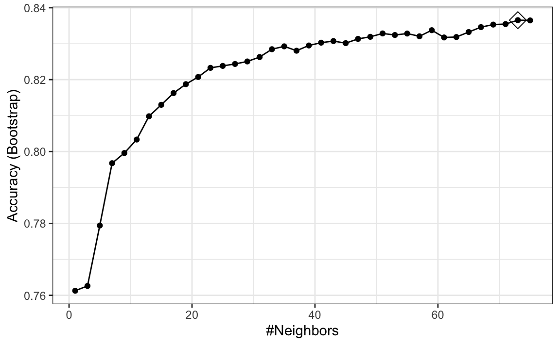
Resampling methods involve random sampling steps, so repeated runs of the same code can produce different outcomes. To ensure results can be reproduced exactly, we set the random seed at the start of the analysis.
The results component of the train output includes several summary statistics related to the variability of the cross-validation estimates:
names(train_knn$results)
#> [1] "k"          "Accuracy"   "Kappa"      "AccuracySD" "KappaSD"
You can learn many more details about the caret package from the manual2.
To access the parameter that maximized the accuracy, you can use this:
train_knn$bestTune
#>     k
#> 41 81
and the best performing model like this:
train_knn$finalModelThe function predict will use this best-performing model. Here is the accuracy of the best model when applied to the test set, which we have not yet used because the cross-validation was done on the training set:
31.2 Case study: handwritten digit recognition
We are now ready to apply these ideas to a real-world example. Throughout this section, we use the MNIST dataset, introduced in Section 21.2, as a case study to illustrate the full modeling workflow.
We load the data using the following function from the dslabs package:
library(dslabs)
mnist <- read_mnist()
The dataset includes two components, a training set and a test set:
names(mnist)
#> [1] "train" "test"
Each of these components includes a matrix with features in the columns:
dim(mnist$train$images)
#> [1] 60000   784
and vector with the classes as integers:
Because we want this example to run on a laptop and in less than one hour, we will consider a subset of the dataset. We will sample 10,000 random rows from the training set and 1,000 random rows from the test set:
But you are welcome to try the ideas on the entire dataset.
When fitting models to large datasets, we recommend using matrices instead of data frames, as matrix operations tend to be faster. In the caret package, predictor matrices must have column names to track features accurately during prediction on the test set. If the matrices lack column names, you can assign names based on their position:
31.3 Preprocessing
We often transform predictors before running machine learning algorithms. We also remove predictors that are clearly not useful. We call these steps preprocessing.
Examples of preprocessing steps include standardizing predictors, applying transformations such as the logarithm, reducing the dimensionality of the feature space, removing highly correlated predictors, and excluding predictors with little variability, for example, those with near-zero variance.
Feature Filtering
As a first example, we focus on this last type of preprocessing by examining the variability of each predictor. Specifically, we compute the standard deviation of each feature and observe that many have values close to zero, indicating minimal variation:
library(matrixStats)
hist(colSds(x), breaks = 256)![]()
This is expected because there are parts of the image that rarely contain writing.
The caret package includes a function that recommends features to be removed due to near-zero variance:
nzv <- nearZeroVar(x)We can see the columns recommended for removal are near the edges:

If we use nearZeroVar, we end up removing length(nzv) = 532 predictors. We can see that the accuracy of kNN is about the same even after removing all these predictors:
The caret package features the preProcess function, which allows users to establish a predefined set of preprocessing operations based on a training set. This function is designed to apply these operations to new datasets without recalculating anything on the validation set, ensuring that all preprocessing steps are consistent and derived solely from the training data.
Below is an example demonstrating how to remove predictors with near-zero variance and then center the remaining predictors:
pp <- preProcess(x, method = c("nzv", "center"))
centered_subsetted_x_test <- predict(pp, newdata = x_test)
Additionally, the train function in caret includes a preProcess argument that allows users to specify which preprocessing steps to apply automatically during model training. Here is an example of how to use it to remove near-zero variance predictors. Because this is an illustrative example, we consider only one \(k\) and use five-fold cross-validation to estimate the MSE to reduce runtime. As we see in Section 31.5, in practice you would want to optimize \(k\) and use more thorough resampling:
knn_nzv <- train(x, y, method = "knn", preProcess = "nzv",
  trControl = trainControl(method = "cv", number = 5),
  tuneGrid = data.frame(k = 5))
mean(predict(knn_nzv, x_test, type = "raw") == y_test)
#> [1] 0.955
Dimension reduction with PCA
An alternative to filtering features directly is to reduce the dimension of the feature matrix using Principal Component Analysis (PCA). For this dataset, a large fraction of the total variability in the predictors can be captured using only a small number of principal components (PCs).
As an example, suppose we want to retain the smallest number of PCs that explain at least 90% of the variability:
We can run an algorithm using only these 87 transformed features. We will use knn3 from the caret package as an example with the default k
knn_pca <- knn3(pca$x[, 1:p], y)A critical point when using PCA for prediction is that the PCA transformation must be learned only from the training set. If we use the validation or test set to compute principal components, or even to compute the means used for centering, we inadvertently leak information from those sets into the training process, leading to overfitting.
To avoid this, we compute the necessary centering and rotation matrices on the training set and then apply the transformation to the test set:
The resulting accuracy is similar to what we obtained with the full feature set, but using only 87 dimensions:
To obtain an unbiased MSE estimate when training with PCA, we must recompute the PCA inside each cross-validation split and apply the resulting transformation to the corresponding validation fold.
Fortunately, the caret package can automate this. The train function includes PCA as one of its available preprocessing steps. We can request PCA with a fixed number of components using
preProcOptions = list(pcaComp = p)
or ask caret to pick the number of components that explain a fixed fraction of variability, such as 90%, using
preProcOptions = list(thresh = 0.9).
Here is how we modify our earlier code to let caret perform PCA during preprocessing:
knn_pca <- train(x, y, method = "knn", preProcess = c("nzv", "pca"),
  trControl = trainControl("cv", n = 20, preProcOptions = list(thresh=0.9)))
This raises a natural question: why did we choose 0.9? Could another threshold lead to better performance?
One limitation of this approach using caret is that we do not automatically optimize the number of PCs. To tune this quantity directly, just like we tune parameters such as \(k\), we would need to define our own model interface. The caret manual3 describes how to build custom models that allow full optimization of the PCA dimension.
31.4 Parallelization
By default, the train function estimates model accuracy using 25 bootstrap resamples. This can be computationally expensive. For example, evaluating 75 values of a tuning parameter requires 25 × 75 = 1,875 model fits, which can take hours for slower algorithms.
A simple way to approximate runtime is to time a single fit and multiply by the total number of fits. For example, with kNN:
system.time(predict(knn3(x[, -nzv], y), newdata = x_test[, -nzv]))
#>    user  system elapsed
#>   2.831   0.047   2.906
On a typical laptop, this takes a few seconds, suggesting the full process could take over an hour.
This cost can be reduced substantially using parallel computing. Modern computers have multiple processors that allow tasks to run simultaneously, and the caret package can take advantage of this. To enable parallelization, we use the doParallel package. We will demonstrate this setup in the next section.
Parallelization can increase memory usage, since each processor may require its own copy of the data. This can be a limitation for large datasets.
31.5 Model tuning and diagnostics
In Sections 29.1 and 30.5, we introduced the k-nearest neighbors (kNN) and random forest algorithms, along with their intuition and formulation. In this section, we use these two methods as working examples to illustrate the process of model selection and tuning. Specifically, we demonstrate how to train and evaluate models in R, choose appropriate hyperparameters, such as \(k\) for kNN and tree-related parameters for random forests, and assess performance using cross-validation.
Optimizing tuning parameters
We start by demonstrating how we select the tuning parameter \(k\) in the kNN algorithm. In caret, this is done using the tuneGrid argument in the train function. The grid of candidate values must be provided as a data frame, with column names matching those returned by modelLookup. For kNN, this means a column named k. The default values are 5, 7, and 9, which is a very limited range.
In practice, selecting the grid and resampling strategy involves a tradeoff. Using fewer cross-validation folds reduces computation time but yields noisier estimates of prediction error, while more folds provide more precise estimates at greater runtime cost.
Because of this tradeoff, it is inefficient to search over a fine grid from the start. Instead, we begin with a coarse grid over a broad range and a faster resampling scheme to identify a promising region. Once we have a rough idea of where the optimal \(k\) lies, we refine the search with a finer grid and more thorough resampling.
Throughout this process, we use parallel computation to reduce runtime, since each combination of tuning parameters and resamples can be evaluated independently. Note that once clusters are registered, the train function automatically uses them for parallel processing, so we do not need to modify our code to take advantage of parallelization.
library(doParallel)
nc <- detectCores() - 1   # it is convention to leave 1 core for the OS
cl <- makeCluster(nc)
registerDoParallel(cl)
set.seed(1991)
knn <- train(x, y, method = "knn", preProcess = c("nzv", "pca"),
                   trControl = trainControl(method = "cv", number = 5,
                           preProcOptions = list(thresh = 0.9)),
                   tuneGrid = data.frame(k = seq(1, 25, 4)))
plot(knn, highlight = TRUE)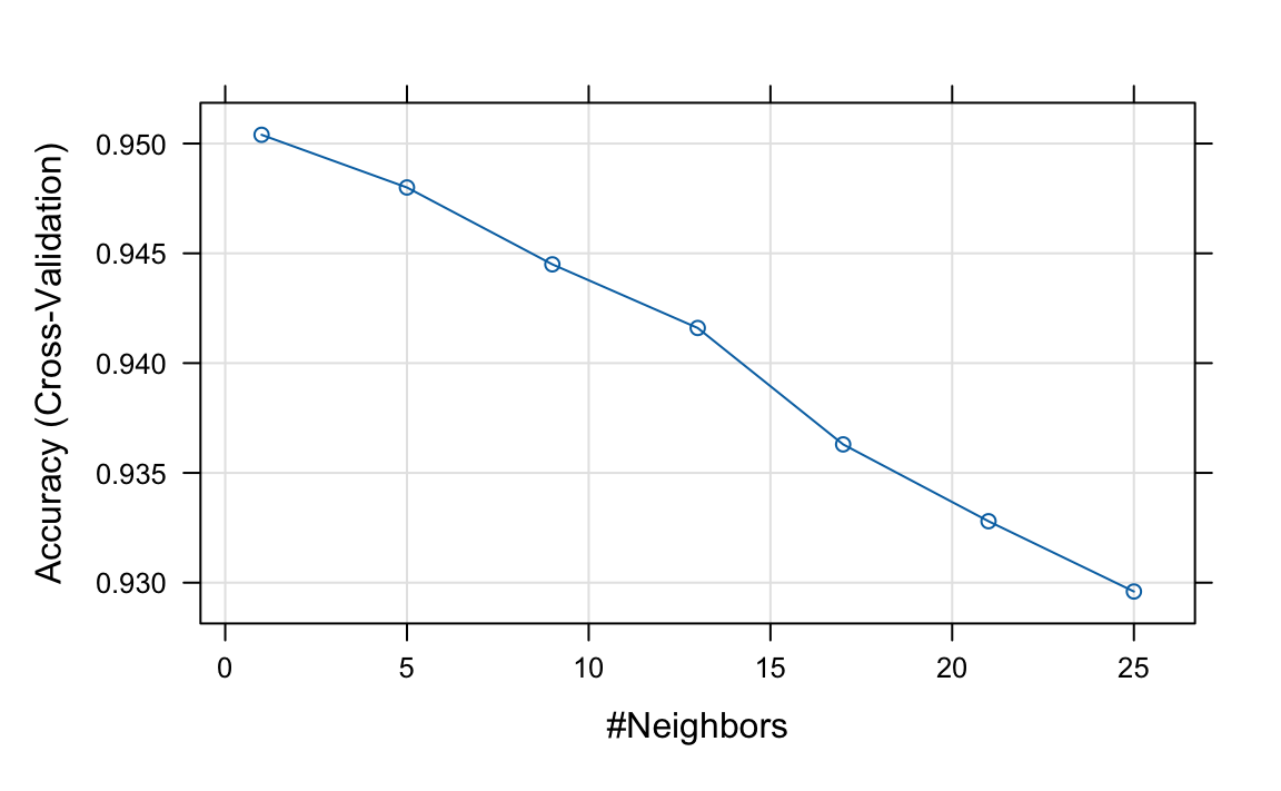
Based on these results, we can infer that the best \(k\) is between 1 and 5. We now refine the search with a finer grid and 20-fold cross-validation:
set.seed(1992)
knn <- train(x, y, method = "knn", preProcess = c("nzv", "pca"),
                   trControl =  trainControl(method = "cv", number = 20,
                           preProcOptions = list(thresh = 0.9)),
                   tuneGrid = data.frame(k = seq(1, 7, 2)))
knn$bestTune
#>   k
#> 2 3
to choose \(k\) = 3. Now that we have optimized our algorithm, the predict function defaults to using the best-performing model fit with the entire training data:
y_hat_knn <- predict(knn, x_test, type = "raw")We achieve relatively high accuracy:
mean(y_hat_knn == y_test)
#> [1] 0.959
Once done with parallelization, it is good practice to stop the cluster:
To verify that parallel processing is active, you can check your system’s process monitor (Activity Monitor, Task Manager, or top) and confirm that multiple R processes are using CPU.
31.6 Improving computational efficiency
With the random forest algorithm, several parameters can be optimized, but the main one is mtry, the number of predictors that are randomly selected for each tree. This is also the only tuning parameter that the caret function train permits when using the default implementation from the randomForest package.
The random forest algorithm is computationally more intensive than kNN and can require substantially longer training times. As a result, tuning its hyperparameters requires a more deliberate strategy. In this example, we adopt several approaches to reduce computation time: we use parallelization, decrease the number of bootstrap resamples, limit the number of trees grown in each fit, and perform an initial search over a coarse grid before refining the search in a narrower region.
We start by fitting the default model and checking
rf <- randomForest(x[, -nzv], y)
plot(rf)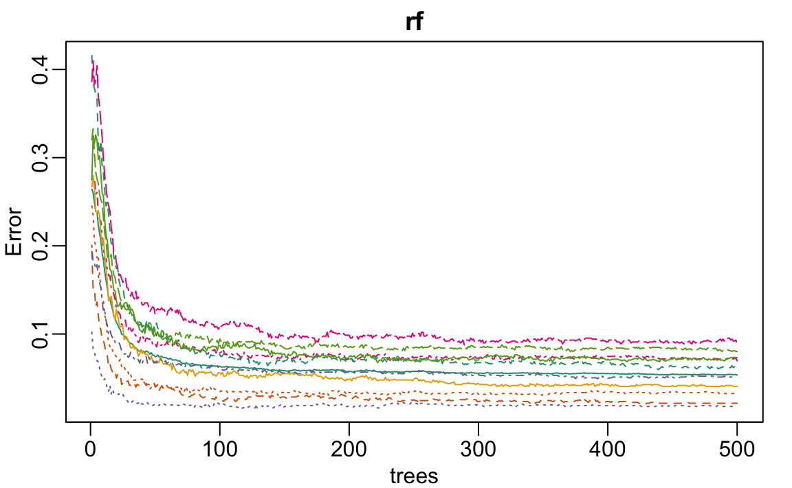
We see that accuracy begins to level off at around 200 trees. So for our coarse search, we limit the number of trees to 200, use five-fold cross-validation instead of 25 bootstrap samples, and consider a coarse grid of mtry values. This reduction in the number of trees and the size of the resampling allows us to reduce the runtime by a factor of 10, which allows us to identify a promising region for mtry relatively quickly:
library(doParallel)
cl <- makeCluster(detectCores() - 1)
registerDoParallel(cl)
set.seed(1993)
rf <- train(x, y, method = "rf", ntree = 250, preProcess = "nzv",
  trControl = trainControl(method = "cv", n = 5),
  tuneGrid = data.frame(mtry = seq(3, 53, 10)))
ggplot(rf, highlight = TRUE)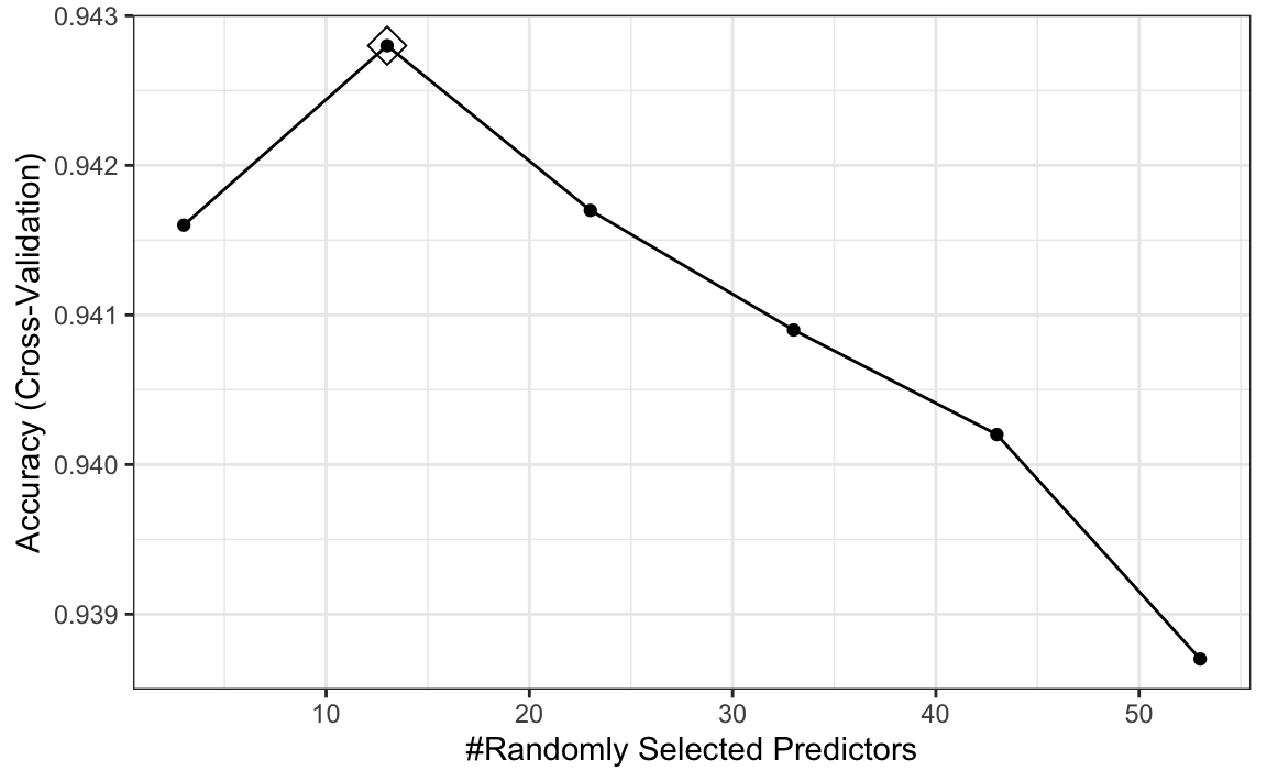
We see that the optimal mtry is between 5 and 20.
Note that with smaller values of mtry, individual trees tend to be weaker because each split considers fewer predictors. As a result, more trees are typically required for performance to stabilize. In contrast, larger values of mtry produce stronger but more correlated trees, so fewer trees may suffice.
When reducing the number of trees to speed up tuning, keep this tradeoff in mind: using too few trees can bias comparisons across mtry values, particularly disadvantaging smaller mtry. It is therefore advisable to use enough trees to obtain stable performance when selecting the range of mtry.
We now refine the search using a finer grid and the default resampling settings. Note that the code below uses 500 trees and 25 bootstrap resamples, so it may take several minutes to run.
set.seed(1994)
rf <- train(x, y, method = "rf", preProcess = "nzv",
  tuneGrid = data.frame(mtry = 5:20))
Now that we have optimized our algorithm, we are ready to predict outcomes with our final model:
y_hat_rf <- predict(rf, x_test, type = "raw")As with kNN, we also achieve high accuracy:
mean(y_hat_rf == y_test)
#> [1] 0.953
Note that by optimizing some of the other algorithm parameters, we could achieve even higher accuracy.
To end, we turn off the use of parallel:
31.7 Diagnostics
An important part of data analysis is visualizing results to better understand our model fit and also determine why we are failing. How we do this depends on the application but below we provide some examples for the example of handwritten digit recognition.
The black box nature of many machine learning algorithms can make it difficult to understand how they are making predictions. However, there are tools available to help us interpret these models and gain insights into their behavior. For example, with random forests we can examine whether variable importance, described in Section 30.5.1, is consistent with our expectations given the context. The following function computes the importance of each feature:
imp <- varImp(rf)$importance[,1]We can see which features are being used most by plotting an image:

A common diagnostic tool is to examine the errors. By looking at the cases where the model made incorrect predictions, we can often identify specific weaknesses in the algorithm or parameter choices and try to correct them. Below we show the images of digits for which we made an incorrect prediction. Here are some errors for the random forest:
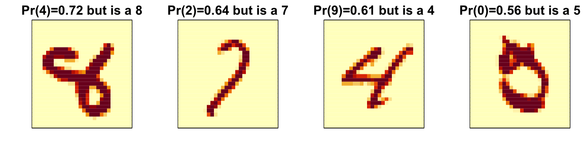
By examining errors like this, we often find specific weaknesses in algorithms or parameter choices and can try to correct them.
31.8 Ensembles
The idea of an ensemble is similar to the idea of combining data from different pollsters to obtain a better estimate of the true support for each candidate.
In machine learning, one can usually greatly improve the final results by combining the results of different algorithms.
Here is a simple example where we compute new class probabilities by taking the average of the previously fitted random forest (saved in rf) and kNN (saved in knn). We can see that the accuracy improves:
We have just built an ensemble with just two algorithms. By combining more similarly performing but uncorrelated algorithms, we can improve accuracy further.
31.9 Exercises
1. Create a simple dataset where the outcome grows 0.75 units on average for every increase in a predictor:
n <- 1000
sigma <- 0.25
x <- rnorm(n, 0, 1)
y <- 0.75 * x + rnorm(n, 0, sigma)
dat <- data.frame(x = x, y = y)
In the exercises in Chapter 30, we saw that changing maxnodes or nodesize in the randomForest function improved our estimate in this dataset. Let’s use the train function to help us pick these values. From the caret manual, we see that we can’t tune the maxnodes parameter or the nodesize argument with randomForest, so we will use the Rborist package and tune the minNode argument. Use the train function to try values minNode <- seq(5, 250, 25). See which value minimizes the estimated RMSE.
2. Make a scatterplot of x and y and add the prediction from the best-fitted model in exercise 1.
3. This dslabs tissue_gene_expression dataset includes a matrix x:
with the gene expression measured on 500 genes for 189 biological samples representing seven different tissues. The tissue type is stored in y:
table(tissue_gene_expression$y)Split the data into training and test sets, then use kNN to predict tissue type and see what accuracy you obtain. Try it for \(k = 1, 3, \dots, 11\).
4. We are going to apply LDA and QDA to the tissue_gene_expression dataset. We will start with simple examples based on this dataset and then develop a realistic example.
Create a dataset with just the classes cerebellum and hippocampus (two parts of the brain) and a predictor matrix with 10 randomly selected columns.
Estimate the accuracy of LDA.
5. In this case, LDA fits two 10-dimensional normal distributions. Look at the fitted model by looking at the finalModel component of the result of train. Notice there is a component called means that includes the estimated means of both distributions. Plot the mean vectors against each other and determine which predictors (genes) appear to be driving the algorithm.
6. Repeat exercises 4 with QDA. Does it have a higher accuracy than LDA?
7. Are the same predictors (genes) driving the algorithm? Make a plot as in exercise 5.
8. One thing we see in the previous plot is that predictors are correlated between groups: some predictors are low in both groups, while others are high in both groups. The mean value of each predictor, colMeans(x), is not informative or useful for prediction, and often it is useful to center or scale each column for interpretation purposes. This can be achieved with the preProcessing argument in train. Re-run LDA with preProcessing = "scale". Note that accuracy does not change, but see how it is easier to identify the predictors that differ more between groups than the plot made in exercise 5.
9. In the previous exercises, we saw that both approaches worked well. Plot the predictor values for the two genes with the largest differences between the two groups in a scatterplot to see how they appear to follow a bivariate distribution as assumed by the LDA and QDA approaches. Color the points by the outcome.
10. Now we are going to increase the complexity of the challenge slightly: we will consider all the tissue types.
What accuracy do you get with LDA?
11. We see that the results are slightly worse. Use the confusionMatrix function to learn what type of errors we are making.
12. Plot an image of the centers of the seven 10-dimensional normal distributions used by the LDA model fit in exercise 10.
13. Use the rpart function to fit a classification tree to the tissue_gene_expression dataset with all genes. That is, redefine
x <- tissue_gene_expression$xUse the train function to estimate the accuracy. Try out cp values of seq(0, 0.05, 0.01). Plot the accuracy to report the results of the best model.
14. Study the confusion matrix for the best-fitting classification tree. What do you observe happening for placenta samples?
15. Notice that placentas are called endometrium more often than placenta. Note also that there are only six placenta samples, and that, by default, rpart requires 20 observations before splitting a node. Thus, it is not possible with these parameters to have a node in which placentas are the majority. Rerun the above analysis, but this time permit rpart to split any node by using the argument control = rpart.control(minsplit = 0). Does the accuracy increase? Look at the confusion matrix again.
16. Plot the tree from the best-fitting model obtained in exercise 13.
17. We can see that with just the genes selected by CART, we are able to predict the tissue type. Now let’s see if we can do even better with a random forest. Use the train function in the caret package and the rf method to train a random forest. Try out values of mtry ranging from, at least, seq(50, 200, 25). What mtry value maximizes accuracy? To permit small nodesize to grow as we did with the classification trees, use the following argument: nodesize = 1. This will take several seconds to run. If you want to test it out, try using smaller values with ntree. Set the seed to 1990.
18. Use the function varImp on the output of train and save it to an object called imp.
19. The rpart model we ran in exercise 15 produced a tree that used just a few predictors. Extracting the predictor names is not straightforward, but can be done. If the output of the call to train was fit_rpart, we can extract the names like this:
ind <- !(fit_rpart$finalModel$frame$var == "<leaf>")
tree_terms <-
  fit_rpart$finalModel$frame$var[ind] |>
  unique() |>
  as.character()
tree_terms
What is the variable importance in the random forest call for these predictors? Where do they rank?
20. Extract the top 50 predictors based on importance, take a subset of x with just these predictors, and apply the function heatmap to see how these genes behave across the tissues. We will introduce the heatmap function in Chapter 32.
21. In Chapter 30, for the 2 or 7 example, we compared the conditional probability \(p(\mathbf{x})\) given two predictors \(\mathbf{x} = (x_1, x_2)^\top\) to the fit \(\hat{p}(\mathbf{x})\) obtained with a machine learning algorithm by making image plots. The following code can be used to make these images and include a curve at the values of \(x_1\) and \(x_2\) for which the predicted conditional probability is \(0.5\):
plot_cond_prob <- function(x_1, x_2, p) {
  data.frame(x_1 = x_1, x_2 = x_2, p = p) |>
    ggplot(aes(x_1, x_2)) +
    geom_raster(aes(fill = p), show.legend = FALSE) +
    stat_contour(aes(z = p), breaks = 0.5, color = "black") +
    scale_fill_gradientn(colors = c("#F8766D", "white", "#00BFC4"))
}
We can see the true conditional probability for the 2 or 7 example like this:
with(mnist_27$true_p, plot_cond_prob(x_1, x_2, p))Fit a kNN model and make this plot for the estimated conditional probability. Hint: Use the argument newdata = mnist_27$train to obtain predictions for a grid of points.
22. Notice that, in the plot made in exercise 21, the boundary is somewhat wiggly. This is because kNN, like the basic bin smoother, does not use a kernel. To improve this, we could try loess. By reading through the available models part of the caret manual, we see that we can use the gamLoess method. We need to install the gam package, if we have not done so already. We see that we have two parameters to optimize:
modelLookup("gamLoess")
#>      model parameter  label forReg forClass probModel
#> 1 gamLoess      span   Span   TRUE     TRUE      TRUE
#> 2 gamLoess    degree Degree   TRUE     TRUE      TRUE
Use resampling to pick a span between 0.15 and 0.75. Keep degree = 1. What span is selected?
23. Show an image plot of the estimate \(\hat{p}(x,y)\) resulting from the model fit in exercise 22. How does the accuracy compare to that of kNN? Comment on the difference between the estimate obtained with kNN.
24. Fit and compare several machine learning models using the mnist_27 training set.
Rather than trying a large number of methods, select a small, diverse subset (for example: knn, gbm, Rborist, svmLinear, avNNet).
Fit each model using train() with default tuning parameters. Compute the accuracy of each model on the test set and compare their performance.
25. Using the models from the previous exercise, build an ensemble prediction based on majority vote.
Compare the ensemble’s accuracy to that of the individual models. Does the ensemble improve performance?
26. Many methods can also produce estimated class probabilities (using type = "prob" in predict).
Construct an ensemble by averaging predicted probabilities across models, then classify using a 0.5 cutoff.
Compare this approach to majority voting. Which performs better?