10 Data-Driven Models
“All models are wrong, but some are useful.” –George E. P. Box
So far, our analysis of poll-related results has been based on a simple sampling model. This model assumes that each voter has an equal chance of being selected for the poll, similar to picking beads from an urn with two colors. However, in this section, we explore real-world data and discover that this model is oversimplified. Instead, we propose a more effective approach in which we directly model the outcomes of pollsters rather than the individual polls.
A more recent development since the original invention of opinion polls is the use of computers to aggregate publicly available data from different sources and develop data-driven forecasting models. Here, we explore how poll aggregators collect and combine data reported by different experts to produce improved predictions. We will introduce ideas behind the statistical models used to improve election forecasts beyond the power of individual polls. Specifically, we introduce a useful model for constructing a confidence interval for the popular vote difference.
It is important to emphasize that this chapter offers only a brief introduction to the vast field of statistical modeling. The model presented here, for example, does not allow us to assign probabilities to outcomes such as a particular candidate winning the popular vote, as is done by poll aggregators like FiveThirtyEight. In the next chapter, we introduce Bayesian models, which provide the mathematical framework for such probabilistic statements. Later, in the Linear Models part of the book, we explore widely used approaches for analyzing data in practice. Still, this introduction only scratches the surface. Readers interested in statistical modeling are encouraged to consult the Recommended Reading section for additional references that provide a deeper and broader perspective.
10.1 Case study: poll aggregators
A few weeks before the 2012 election, Nate Silver was giving Obama a 90% chance of winning. How was Mr. Silver so confident? We will use a Monte Carlo simulation to illustrate the insight Mr. Silver had, and which others missed.
A Monte Carlo simulation
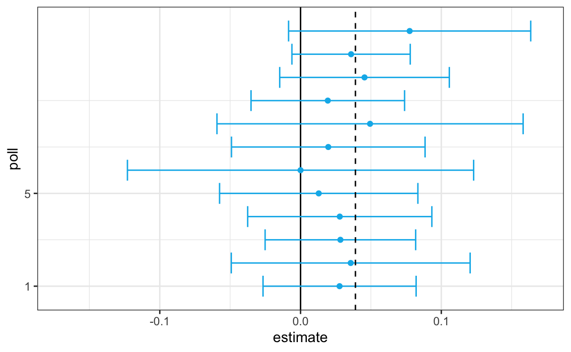
To do this, we simulate results for 12 polls taken the week before the election. We mimic sample sizes from actual polls, construct, and report 95% confidence intervals for the spread for each of the 12 polls:
Not surprisingly, all 12 polls report confidence intervals that include the result we eventually saw on election night (vertical dashed line). However, all 12 polls also include 0 (vertical solid line). Therefore, if asked individually for a prediction, the pollsters would have to say: it’s a toss-up.
Poll aggregators recognized that combining results from multiple polls can greatly improve precision. One straightforward approach is to reverse engineer the original data from each poll using the reported estimates and sample sizes. From these, we can reconstruct the total number of successes and failures across all polls, effectively combining them into a single, larger dataset. We then compute a new overall estimate and its corresponding standard error using the combined sample size, which is much larger than that of any individual poll.
When we do this, the resulting margin of error is 0.018.
Our combined estimate predicts a spread of 3.1 percentage points, plus or minus 1.8. This interval not only includes the actual result observed on election night but is also far from including zero. By aggregating the twelve polls, assuming no systematic bias, we obtain a much more precise estimate and can be quite confident that Obama will win the popular vote.

However, this example was just a simplified simulation to illustrate the basic idea. In real-world settings, combining data from multiple polls is more complicated than treating them as one large random sample. Differences in methodology, timing, question wording, and even sampling biases can all affect the results. We will later explore how these factors make real poll aggregation more challenging and how statistical models can account for them.
Real data from the 2016 presidential election
The following subset of the polls_us_election_2016 data in dslabs includes results for national polls as well as state polls taken during the year prior to the election and organized by FiveThirtyEight. In this first example, we will filter the data to include national polls conducted on likely voters (lv) within the last week leading up to the election and consider their estimate of the spread:
Note that we will focus on predicting the spread, not the proportion \(p\). Since we are assuming there are only two parties, we know that the spread is \(\theta = p - (1-p) = 2p - 1\). As a result, everything we have done can easily be adapted to an estimate of \(\theta\). Once we have our estimate \(\bar{X}\) and \(\widehat{\mathrm{SE}}[\bar{X}]\), we estimate the spread with \(2\bar{X} - 1\) and, since we are multiplying by 2, the standard error is \(2\widehat{\mathrm{SE}}[\bar{X}]\). Remember that subtracting 1 does not add any variability, so it does not affect the standard error. Also, the CLT applies here because our estimate is a linear combination of a sample average, which itself follows approximately normal distributions.
We use \(\theta\) to denote the spread here because this is a common notation used in statistical textbooks for the parameter of interest.
We have 50 estimates of the spread. The theory we learned from sampling models tells us that these estimates are realizations of a random variable with a probability distribution that is approximately normal. The expected value is the election night spread \(\theta\), and the standard error is \(2\sqrt{p (1 - p) / N}\).
Assuming the urn model we described earlier is a good one, we can use this information to construct a confidence interval based on the aggregated data. The estimated spread is:
and the standard error is:
So we report a spread of 3.59% with a margin of error of 0.4%. On election night, we discover that the actual percentage was 2.1%, which is outside a 95% confidence interval. What happened?
A histogram of the reported spreads reveals a problem:
The estimates do not appear to be normally distributed, and the standard error appears to be larger than 0.0038. The theory is not working here.
10.2 Beyond the simple sampling model
Notice that data come from various pollsters, and some are taking several polls a week:
polls |> count(pollster) |> arrange(desc(n)) |> head(5)
#>                   pollster n
#> 1                 IBD/TIPP 6
#> 2 The Times-Picayune/Lucid 6
#> 3    USC Dornsife/LA Times 6
#> 4 ABC News/Washington Post 5
#> 5     CVOTER International 5
Let’s visualize the data for the pollsters that are regularly polling:

This plot reveals an unexpected result. First, consider that the standard error predicted by theory for each poll is between 0.018 and 0.033:
polls |> group_by(pollster) |> filter(n() >= 5) |>
  summarize(se = 2*sqrt(p_hat*(1 - p_hat)/median(samplesize)))
#> # A tibble: 5 × 2
#>   pollster                     se
#>   <fct>                     <dbl>
#> 1 ABC News/Washington Post 0.0243
#> 2 CVOTER International     0.0260
#> 3 IBD/TIPP                 0.0333
#> 4 The Times-Picayune/Lucid 0.0197
#> 5 USC Dornsife/LA Times    0.0183
This agrees with the within-poll variation we see. However, there appear to be differences across the polls. Observe, for example, how the USC Dornsife/LA Times pollster is predicting a 4% lead for Trump, while Ipsos is predicting a lead larger than 5% for Clinton. The theory we learned says nothing about different pollsters producing polls with different expected values; instead, it assumes all the polls have the same expected value. FiveThirtyEight refers to these differences as house effects. We also call it pollster bias. Nothing in our simple urn model provides an explanation for these pollster-to-pollster differences.
This model misspecification led to an overconfident interval that ended up not including the election night result. So, rather than modeling the process generating these values with an urn model, we instead model the pollster results directly. To do this, we collect data. Specifically, for each pollster, we look at the last reported result before the election:
one_poll_per_pollster <- polls |> group_by(pollster) |>
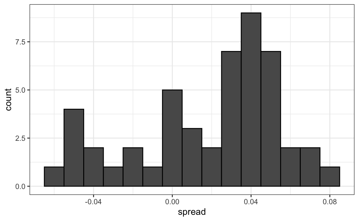
slice_max(enddate, n = 1, with_ties = FALSE) |> ungroup()Here is a histogram of the calculated spread for these 20 pollsters’ final polls:
hist(one_poll_per_pollster$spread, breaks = 10)
Although we are no longer using a model with red (Republicans) and blue (Democrats) beads in an urn, our new model can also be thought of as an urn model, but containing poll results from all possible pollsters. Think of our \(N=\) 20 data points \(Y_1,\dots Y_N\) as a random sample from this urn. To develop a useful model, we assume that the expected value of our urn is the actual spread \(\theta = 2p - 1\), which implies that the sample average has expected value \(\theta\).
Now, instead of 0s and 1s, our urn contains continuous numbers representing poll results. The standard deviation of this urn is therefore no longer \(2\sqrt{p(1-p)}\). In this setting, the variability we observe arises not only from random sampling of voters but also from differences across pollsters. Our new urn captures both sources of variation. The overall standard deviation of this distribution is unknown, and we denote it by \(\sigma\).
So our new statistical model is that \(Y_1, \dots, Y_N\) are a random sample with expected \(\theta\) and standard deviation \(\sigma\). The distribution, for now, is unspecified. But we consider \(N\) to be large enough to assume that the sample average \(\bar{Y} = \sum_{i=1}^N Y_i\) follows a normal distribution with expected value \(\theta\) and standard error \(\sigma / \sqrt{N}\) under the CLT. We write:
\[ \bar{Y} \sim \mbox{N}(\theta, \sigma / \sqrt{N}) \]
Here, the \(\sim\) symbol tells us that the random variable on the left of the symbol follows the distribution on the right. We use the notation \(N(a,b)\) to represent the normal distribution with mean \(a\) and standard deviation \(b\).
This model for the sample average will be used again in the next chapter.
Estimating the standard deviation
The model we have specified has two unknown parameters: the expected value \(\theta\) and the standard deviation \(\sigma\). We know that the sample average \(\bar{Y}\) will be our estimate of \(\theta\). But what about \(\sigma\)?
Our task is to estimate \(\theta\). Given that we model the observed values \(Y_1,\dots Y_N\) as a random sample from the urn, for a large enough sample size \(N\), the probability distribution of the sample average \(\bar{Y}\) is approximately normal with expected value \(\theta\) and standard error \(\sigma/\sqrt{N}\). If we are willing to consider \(N=\) 20 large enough, we can use this to construct confidence intervals.
Theory tells us that we can estimate the urn model \(\sigma\) with the sample standard deviation defined as:
\[ s = \sqrt{ \frac{1}{N-1} \sum_{i=1}^N (Y_i - \bar{Y})^2 } \]
Keep in mind that, unlike for the population standard deviation definition, we now divide by \(N-1\). This makes \(s\) a better estimate of \(\sigma\). There is a mathematical explanation for this, which is explained in most statistics textbooks, but we do not cover it here.
The sd function in R computes the sample standard deviation:
sd(one_poll_per_pollster$spread)
#> [1] 0.0222
Computing a confidence interval
We are now ready to form a new confidence interval based on our new data-driven model:
Our confidence interval is wider now since it incorporates the pollster variability. It does include the election night result of 2.1%. Also, note that it was small enough not to include 0, which means we were confident Clinton would win the popular vote.
The t-distribution
Above, we made use of the CLT with a sample size of 20. Because we are estimating a second parameter \(\sigma\), further variability is introduced into our confidence interval, which results in intervals that are too small. For very large sample sizes, this extra variability is negligible, but in general, especially for \(N\) smaller than 30, we need to be cautious about using the CLT.
Note that 30 is a very general rule of thumb based on the case when the data come from a normal distribution. There are cases when a larger sample size is needed, as well as cases when smaller sample sizes are good enough.
However, if the data in the urn is known to follow a normal distribution, then we actually have mathematical theory that tells us how much bigger we need to make the intervals to account for the estimation of \(\sigma\). Applying this theory, we can construct confidence intervals for any \(N\). But again, this works only if the data in the urn is known to follow a normal distribution. So, for the 0, 1 data of our previous urn model, this theory definitely does not apply.
The statistic on which confidence intervals for \(\theta\) are based is:
\[ Z = \frac{\bar{Y} - \theta}{\sigma/\sqrt{N}} \] Here, \(\theta\) is the true population spread, and \(\sigma\) is the standard deviation of the pollster-level urn.
CLT tells us that Z is approximately normally distributed with expected value 0 and standard error 1. But in practice we don’t know \(\sigma\), so we use:
\[ t = \frac{\bar{Y} - \theta}{s/\sqrt{N}} \]
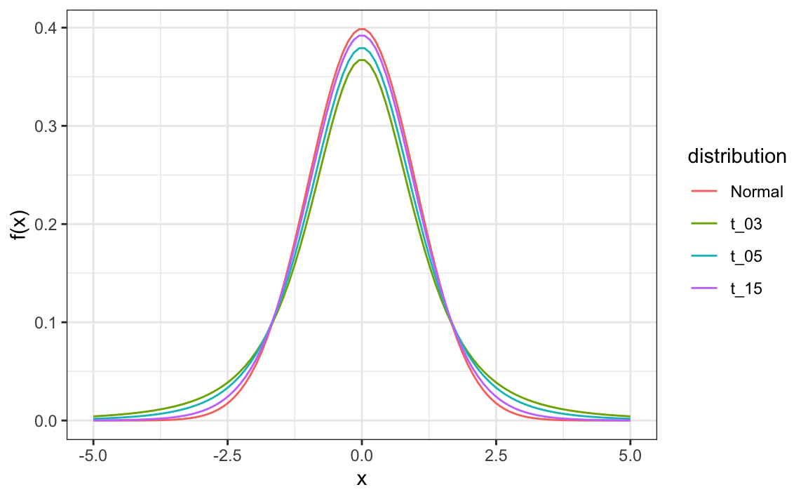
This is referred to as a t-statistic. By substituting \(\sigma\) with \(s\), we introduce some variability. The theory tells us that \(t\) follows a Student’s t-distribution with \(N-1\) degrees of freedom. The degrees of freedom is a parameter that controls the variability via fatter tails. Here are three examples of t-distributions with three different degrees of freedom:
If we are willing to assume the pollster effect data is normally distributed, based on the sample data \(Y_1, \dots, Y_N\),
one_poll_per_pollster |> ggplot(aes(sample = spread)) + stat_qq()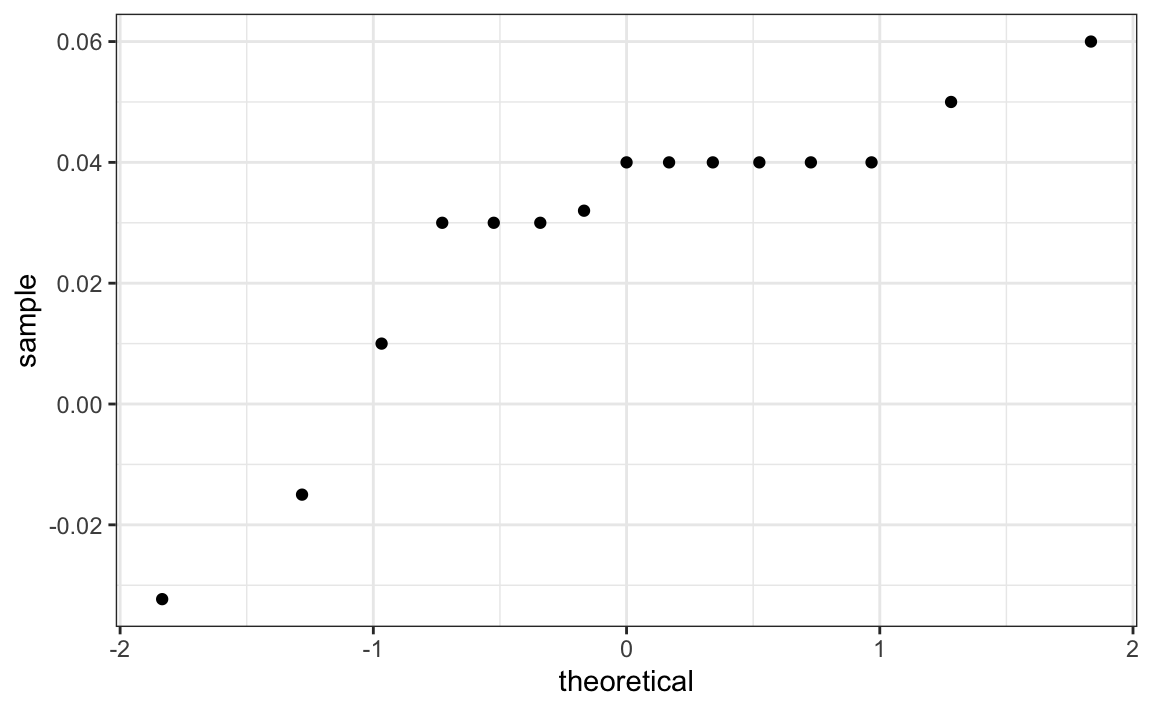
then \(t\) follows a t-distribution with \(N-1\) degrees of freedom.
Using the t-distribution and the t-statistic is the basis for t-tests, a widely used approach for computing p-values. To learn more about t-tests, you can consult any statistics textbook.
To construct a 95% confidence interval, we simply use qt instead of qnorm. This results in a slightly larger confidence interval than we obtained before:
n <- length(one_poll_per_pollster$spread)
t_crit <- qt(0.975, n - 1)
ttest_ci <- one_poll_per_pollster |>
  summarize(avg = mean(spread), se = sd(spread)/sqrt(length(spread))) |>
  mutate(start = avg - t_crit*se, end = avg + t_crit*se) |>
  select(start, end)
round(ttest_ci*100, 2)
#>   start  end
#> 1  1.99 4.07
This interval is a bit larger than the one using normal because the t-distribution has large tails, as seen in the densities. Specifically, the 97.5th quantile value for the t distribution
qt(0.975, n - 1)
#> [1] 2.09
is larger than that for the normal distribution
qnorm(0.975)
#> [1] 1.96
The t-distribution approximation used for confidence intervals and hypothesis tests is exact only when the data are normally distributed. However, in practice, it works quite well more broadly. When the distribution of the data is unimodal and approximately symmetric, the t-based methods continue to give accurate results even if the data are not perfectly normal.
This guidance is intentionally imprecise. With experience, you develop a sense for when the approximation is reliable. When the shape of the data is unclear, Monte Carlo simulations provide a practical check: you can simulate repeated samples under a proposed model and examine whether the resulting confidence interval or test behaves as expected.
In short, normality is not required, but strong skew or heavy tails can break the approximation, so always look at the data.
The t-distribution can also be used to model errors in bigger deviations that are more likely than with the normal distribution. In their Monte Carlo simulations, FiveThirtyEight uses the t-distribution to generate errors that better model the deviations we see in election data. For example, in Wisconsin, the average of six high-quality polls was 7% in favor of Clinton with a standard deviation of 3%, but Trump won by 0.8%. Even after taking into account the overall bias, this 7.7% residual is more in line with t-distributed data than the normal distribution.
10.3 Exercises
We have been using urn models to motivate the use of probability models. Yet, most data science applications are not related to data obtained from urns. More common are data that come from individuals. The reason probability plays a role here is that the data come from a random sample. The random sample is taken from a population, and the urn serves as an analogy for the population.
To answer the following questions, define the males who replied to the height survey as the population:
1. Mathematically speaking, x is our population. Using the urn analogy, we have an urn with the values of x in it. What are the mean and standard deviation of our population?
2. Call the population mean computed above \(\mu\) and the standard deviation \(\sigma\). Now take a sample of size 50, with replacement, and construct an estimate for \(\mu\) and \(\sigma\).
3. What does the theory tell us about the sample average \(\bar{X}\) and how it is related to \(\mu\)?
- It is practically identical to \(\mu\).
- It is a random variable with expected value \(\mu\) and standard error \(\sigma/\sqrt{N}\).
- It is a random variable with expected value \(\mu\) and standard error \(\sigma\).
- Contains no information.
4. So, how is this useful? We are going to use an oversimplified yet illustrative example. Suppose we want to know the average height of our male students, but we can only measure 50 of the 708. We will use \(\bar{X}\) as our estimate. We know from the answer to exercise 3 that the standard error of our error \(\bar{X}-\mu\) is \(\sigma/\sqrt{N}\). We want to compute this, but we don’t know \(\sigma\). Based on what is described in this chapter, show your estimate of \(\sigma\).
5. Construct a 95% confidence interval for \(\mu\) using our estimate of \(\sigma\).
6. Now run a Monte Carlo simulation in which you compute 10,000 confidence intervals as you did in exercise 5. What proportion of these intervals include \(\mu\)?
7. Use the qnorm and qt functions to generate quantiles. Compare these quantiles for different degrees of freedom for the t-distribution. Use this to motivate the sample size of 30 rule of thumb.