x_hat <- 0.48
se <- sqrt(x_hat*(1 - x_hat)/25)
se
#> [1] 0.099910 Confidence Intervals
Pollsters summarize uncertainty using a single, easy-to-interpret number called the margin of error. The margin of error, together with the estimate of the parameter, allows them to report an interval that they are confident contains the true value. But what does confident actually mean?
To connect this idea to a familiar challenge, consider the competition described in Section 9.1, where you were asked to report an interval for the true proportion \(p\). If your interval included the actual \(p\), you recovered half the cost of your poll and advanced to the next round. A guaranteed way to move on would be to report a very wide interval,say \([0,1]\), which is certain to contain \(p\). But such an interval is useless: it conveys no information, and you would very likely lose to someone submitting a shorter interval. Similarly, an election forecaster who predicts that the spread will be between −100% and 100% would not be taken seriously. Even an interval between −10% and 10% would be too vague to be meaningful.
On the other hand, a very narrow interval is risky. A pollster who reports extremely tight intervals but frequently misses the true value will quickly lose credibility. The goal is to find a balance: intervals that are narrow enough to be informative but wide enough to be reliable.
Statistical theory provides a way to quantify precisely what we mean by confidence, using the probability framework developed earlier. Specifically, we can construct intervals for which we can compute the probability of containing the true parameter \(p\). When a pollster reports an estimate along with a margin of error, they are effectively reporting an interval with a 95% probability of containing the true parameter, known as a 95% confidence interval.
In this chapter, we show how to construct and interpret such confidence intervals.
10.1 The Central Limit Theorem
In Chapter 9, we introduced the sample average \(\bar{X}\) as an estimate of the parameter \(p\), and we showed how to compute its standard error. However, to calculate probabilities, we need more, we need the probability distribution of \(\bar{X}\).
In the Probability part of the book (Section 8.3), we learned that when the sample size is large, the average of independent draws from a population is approximately normally distributed, regardless of the shape of the population. This is the Central Limit Theorem (CLT). Because \(\bar{X}\) is itself the average of independent draws, the CLT applies directly here, and it is the main tool used to construct confidence intervals.
Let’s use it to answer a concrete question:
How likely is it that our sample estimate \(\bar{X}\) is within 2% of the true population proportion \(p\)?
We can express this as:
\[ \Pr(|\bar{X} - p| \leq 0.02) = \Pr(\bar{X} \leq p + 0.02) - \Pr(\bar{X} \leq p - 0.02). \]
If we standardize \(\bar{X}\), that is, subtract its expected value and divide by its standard error, we obtain a standard normal random variable which we will call \(Z\):
\[ Z = \frac{\bar{X} - \mathrm{E}[\bar{X}]}{\mathrm{SE}[\bar{X}]}. \]
Since \(\mathrm{E}[\bar{X}] = p\) and \(\mathrm{SE}[\bar{X}] = \sqrt{p(1-p)/N}\), the probability above becomes:
\[ \Pr\!\left(Z \leq \frac{0.02}{\sqrt{p(1-p)/N}}\right) - \Pr\!\left(Z \leq -\frac{0.02}{\sqrt{p(1-p)/N}}\right). \]
To compute this, we need \(\sqrt{p(1-p)/N}\), but \(p\) is unknown. Fortunately, the CLT still holds if we use a plug-in estimate, replacing \(p\) with our observed \(\bar{X}\):
\[ \widehat{\mathrm{SE}}[\bar{X}] = \sqrt{\bar{X}(1 - \bar{X})/N}. \]
In statistics, hats indicate estimates. For example, \(\hat{p}\) is often used instead of \(\bar{X}\) to denote the estimate of \(p\). Similarly, \(\widehat{\mathrm{SE}}\) means we are estimating the standard error rather than computing it exactly.
Using our earlier poll with \(\bar{X} = 0.48\) and \(N = 25\), we obtain:
Now we can compute the probability that our estimate is within 2% of the true value:
There’s only a small chance of being this close when \(N = 25\).
The same reasoning applies for any desired error. For example, to find the probability that \(\bar{X}\) is within error of \(p\), we compute:
We can also reverse the question: What value of error gives a 95% probability that \(\bar{X}\) is within that range of \(p\)?
Mathematically, we solve for \(\epsilon\) in:
\[ \Pr(|\bar{X} - p| \leq \epsilon) = 0.95. \]
Following the same logic, this is equivalent to finding the value of error for which pnorm(error/se) - pnorm(-error/se) = 0.95. Because:
we find that \(\epsilon = 1.96 \times \widehat{\mathrm{SE}}[\bar{X}]\).
In the next section, we use this result, derived from the CLT, to construct confidence intervals that capture the true parameter with a specified level of probability.
10.2 Constructing Confidence Intervals
In the previous section, we showed that the interval
\[\left[\bar{X} - 1.96,\widehat{\mathrm{SE}}[\bar{X}], \bar{X} + 1.96,\widehat{\mathrm{SE}}[\bar{X}]\right]\]
has a 95% probability of containing the true proportion \(p\). This type of interval is called a 95% confidence interval. Let’s take a closer look at what that statement really means.
The endpoints of this interval are not fixed numbers, they depend on the data. Each time we take a new sample, we obtain a new \(\bar{X}\) and thus a new confidence interval. To see this, we can repeat the sampling process using the same parameters as before:
If you run this code several times, you’ll see that the interval changes from run to run due to random sampling variation.
The definition of a 95% confidence interval is that, over many repetitions of this process, approximately 95% of the intervals constructed in this way will contain the true value of \(p\). We can verify this mathematically by reversing the derivation from the previous section:
\[ \begin{aligned} \Pr\!\left(p \in \left[\bar{X} - 1.96 \,\widehat{\mathrm{SE}}[\bar{X}], \bar{X} + 1.96\,\widehat{\mathrm{SE}}[\bar{X}]\right]\right) &= \Pr\!\left(\bar{X} - 1.96\,\widehat{\mathrm{SE}}[\bar{X}] \leq p \leq \bar{X} + 1.96\,\widehat{\mathrm{SE}}[\bar{X}]\right)\\ &= \Pr\!\left(-1.96 \leq \frac{\bar{X} - p}{\widehat{\mathrm{SE}}[\bar{X}]} \leq 1.96\right) \\ &= \Pr(-1.96 \leq Z \leq 1.96) \end{aligned} \]
where \(Z\) is a standard normal random variable. Using R:
we confirm that this probability is 0.95.
The interval we derived is not the only one with a 95% probability of containing \(p\). More precisely, we constructed the 95% confidence interval centered at \(\bar{X}\). While it may seem intuitive to center the interval at the estimate rather than use an asymmetric interval with \(\bar{X}\) near one edge, there is mathematical justification for this choice. Statistical theory shows that the symmetric interval centered at \(\bar{X}\) is the shortest interval that achieves 95% coverage of \(p\) under standard assumptions.
If we want greater confidence, say 99%, we need to extend the interval further, using the value of \(z\) that satisfies
\[ \Pr(-z \leq Z \leq z) = 0.99. \]
In R, we can find this value with:
z <- qnorm(0.995)By definition, pnorm(qnorm(0.995)) = 0.995, and by symmetry, pnorm(-qnorm(0.995)) = 0.005. Thus,
yields 0.995 - 0.005 = 0.99.
This logic works for any desired level of confidence. In general, textbooks express the confidence level as \(1 - \alpha\). The corresponding \(z\)-value satisfies \(z = \Phi^{-1}(1-\alpha/2)\) or:
z <- qnorm(1 - alpha/2)since the area between \(-z\) and \(z\) under the standard normal curve is \(1 - \alpha\).
For example, with \(\alpha = 0.05\) (a 95% confidence level), we have \(1 - \alpha/2 = 0.975\), and:
qnorm(0.975)
#> [1] 1.96
which gives the familiar value 1.96 used earlier.
10.3 A Monte Carlo Simulation
We can confirm that the intervals we construct have the desired probability of including \(p\) empirically using a Monte Carlo simulation. Specitically, by repeatedly drawing samples and constructing confidence intervals, we can check how often the intervals actually contain the true value of \(p\).
As expected, the interval covers \(p\) about 95% of the time.
The plot below shows the first 100 simulated confidence intervals. Each horizontal line represents one interval, and the black vertical line marks the true proportion \(p\). Notice that roughly 95% of the intervals overlap the line, while about 5% miss it, just as the theory predicts.
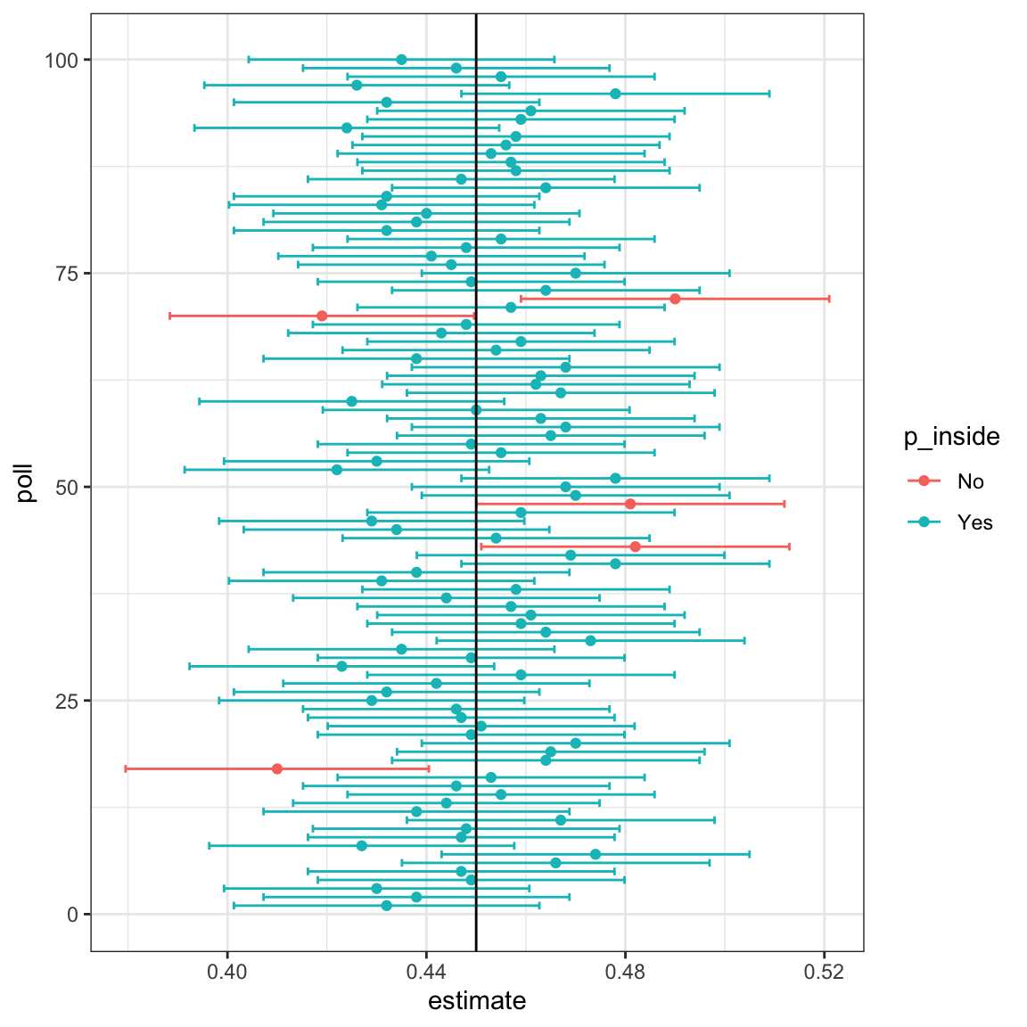
When applying the theory described above, remember that the intervals are random, not \(p\). In the plot above, the confidence intervals vary across samples, but the true proportion \(p\), shown as a vertical line, remains fixed. The “95%” refers to the probability that a randomly constructed interval will cover \(p\).
It is therefore incorrect to say that “\(p\) has a 95% chance of being between these values”, because \(p\) is not random, it is a fixed quantity. The randomness lies in the data and, consequently, in the intervals we compute from the data.
10.4 Margin of Error
We began this chapter by discussing margins of error. How do they relate to confidence intervals? The connection is simple: the margin of error is the value that, when added to and subtracted from the estimate, produces a 95% confidence interval.
Some pollsters use different confidence levels, such as 90% or 99%, which lead to smaller or larger margins of error, respectively. However, 95% is by far the most common and can be assumed unless stated otherwise.
For polls, the margin of error is given by:
\[ 1.96 \sqrt{\hat{X}(1-\hat{X}) / N}. \]
To increase confidence, we can widen the interval (increasing the 1.96 multiplier) or collect a larger sample (increasing \(N\)). Conversely, for a fixed level of confidence, increasing the sample size reduces the margin of error.
Why not just run a huge poll?
In our example, if we surveyed 100,000 people, the margin of error would shrink to less than 0.3%:
In fact, we can make the margin of error as small as we want by increasing \(N\).
So why don’t pollsters do this?
Cost is one reason, but an even more important one is bias. Real-world polls are rarely simple random samples. Some people decline to respond, others may misreport their preferences, and many are simply unreachable. Furthermore, defining the population itself, eligible voters, registered voters, or likely voters, is not straightforward.
These imperfections introduce systematic errors that the margin of error does not capture. Historically, U.S. popular-vote polls have shown biases of about 2-3%. Understanding and modeling these biases is an essential part of modern election forecasting, a topic we will revisit in the next changer (Chapter 11).
10.5 Exercises
1. Write an urn model function that takes the proportion of Democrats \(p\) and the sample size \(N\) as arguments, and returns the sample average if Democrats are 1s and Republicans are 0s. Call the function take_sample.
2. Now assume p <- 0.45 and that your sample size is \(N=100\). Take a sample 10,000 times and save the vector of mean(X) - p into an object called errors. Hint: Use the function you wrote for exercise 1 to write this in one line of code.
3. The vector errors contains, for each simulated sample, the difference between the actual \(p\) and our estimate \(\bar{X}\). We refer to this difference as the error. Compute the average and make a histogram of the errors generated in the Monte Carlo simulation, and select which of the following best describes their distributions:
- The errors are all about 0.05.
- The errors are all about -0.05.
- The errors are symmetrically distributed around 0.
- The errors range from -1 to 1.
4. Note that the error \(\bar{X}-p\) is a random variable. In practice, the error is not observed because we do not know \(p\). Here, we observe it since we constructed the simulation. What is the average size of the error if we define the size by taking the absolute value \(\mid \bar{X} - p \mid\)?
5. The standard error is related to the typical size of the error we make when predicting. For mathematical reasons related to the Central Limit Theorem, we actually use the standard deviation of errors, rather than the average of the absolute values, to quantify the typical size. What is this standard deviation of the errors?
6. The theory we just learned tells us what this standard deviation is going to be because it is the standard error of \(\bar{X}\). What does theory tell us is the standard error of \(\bar{X}\) for a sample size of 100?
7. In practice, we don’t know \(p\), so we construct an estimate of the theoretical prediction by plugging in \(\bar{X}\) for \(p\). Compute this estimate. Set the seed at 1 with set.seed(1).
8. Note how close the standard error estimates obtained from the Monte Carlo simulation (exercise 5), the theoretical prediction (exercise 6), and the estimate of the theoretical prediction (exercise 7) are. The theory is working and it gives us a practical approach to knowing the typical error we will make if we predict \(p\) with \(\bar{X}\). Another advantage that the theoretical result provides is that it gives an idea of how large a sample size is required to obtain the precision we need. Earlier, we learned that the largest standard errors occur for \(p=0.5\). Create a plot of the largest standard error for \(N\) ranging from 100 to 5,000. Based on this plot, how large does the sample size have to be to have a standard error of about 1%?
- 100
- 500
- 2,500
- 4,000
9. For sample size \(N=100\), the Central Limit Theorem tells us that the distribution of \(\bar{X}\) is:
- practically equal to \(p\).
- approximately normal with expected value \(p\) and standard error \(\sqrt{p(1-p)/N}\).
- approximately normal with expected value \(\bar{X}\) and standard error \(\sqrt{\bar{X}(1-\bar{X})/N}\).
- not a random variable.
10. Based on the answer from exercise 8, the error \(\bar{X} - p\) is:
- practically equal to 0.
- approximately normal with expected value \(0\) and standard error \(\sqrt{p(1-p)/N}\).
- approximately normal with expected value \(p\) and standard error \(\sqrt{p(1-p)/N}\).
- not a random variable.
11. To corroborate your answer to exercise 9, make a qq-plot of the errors you generated in exercise 2 to see if they follow a normal distribution.
12. If \(p=0.45\) and \(N=100\) as in exercise 2, use the CLT to estimate the probability that \(\bar{X}>0.5\). Assume you know \(p=0.45\) for this calculation.
13. Assume you are in a practical situation and you don’t know \(p\). Take a sample of size \(N=100\) and obtain a sample average of \(\bar{X} = 0.51\). What is the CLT approximation for the probability that your error is equal to or larger than 0.01?
For the next exercises, we will use actual polls from the 2016 election included in the dslabs package. Specifically, we will use all the national polls that ended within one week prior to the election.
14. For the first poll, you can obtain the samples size and estimated Clinton percentage with:
N <- polls$samplesize[1]
x_hat <- polls$rawpoll_clinton[1]/100
Assume there are only two candidates and construct a 95% confidence interval for the election night proportion \(p\).
15. Now use dplyr to add a confidence interval as two columns, call them lower and upper, to the object polls. Then, use select to show the pollster, enddate, x_hat,lower, upper variables. Hint: Define temporary columns x_hat and se_hat.
16. The final tally for the popular vote was Clinton 48.2% and Trump 46.1%. Add a column, call it hit, to the previous table stating if the confidence interval included the true proportion \(p=0.482\) or not.
17. For the table you just created, what proportion of confidence intervals included \(p\)?
18. If these confidence intervals are constructed correctly, and the theory holds up, what proportion should include \(p\)?
19. A much smaller proportion of the polls than expected produce confidence intervals containing \(p\). If you look closely at the table, you will see that most polls that fail to include \(p\) are underestimating. The main reason for this is undecided voters, individuals polled that do not yet know who they will vote for or do not want to say. Because, historically, undecideds divide evenly between the two main candidates on election day, it is more informative to estimate the spread or the difference between the proportion of two candidates, \(\theta\), which in this election was \(0. 482 - 0.461 = 0.021\). Assume that there are only two parties and that \(\theta = 2p - 1\). Redefine polls as below and re-do exercise 15, but for the difference.
20. Now repeat exercise 16, but for the difference.
21. Now repeat exercise 17, but for the difference.
22. Although the proportion of confidence intervals increases substantially, it is still lower than 0.95. In the next chapter, we learn the reason for this. To motivate this, make a plot of the error, the difference between each poll’s estimate and the actual \(\theta=0.021\). Stratify by pollster.
23. Redo the plot that you made for exercise 22, but only for pollsters that took five or more polls.