
21 Working with Matrices in R
When the number of variables associated with each observation is large, and they can all be represented as numbers, it is often more convenient to store the data in a matrix and perform the analysis using linear algebra, rather than storing the data in a data frame and using tidyverse or data.table functions. Matrix operations form the computational foundation for many applications of linear algebra in data analysis.
In fact, many of the most widely used machine learning algorithms, including linear regression, principal component analysis, neural networks, and deep learning, are built around linear algebra concepts, and their implementations rely heavily on efficient matrix operations. Becoming fluent in creating, manipulating, and interpreting matrices in R will make it easier to understand and implement these methods in practice.
Although we introduce the mathematical framework of linear algebra in the next chapter, the examples we use there rely on being able to work with matrices in R. Therefore, before diving into the mathematical concepts, we begin here with the tools needed to create and operate on matrices in R.
In Section 21.5, at the end of the chapter, we present motivating examples and specific practical tasks that commonly arise in machine learning workflows, such as centering and scaling variables, computing distances, and applying linear transformations. These tasks can be completed efficiently using matrix operations, and the skills you develop in the earlier sections of the chapter will help you solve them. If you would like to understand the motivation for learning the matrix operations introduced in the previous sections, you may find it helpful to read Section 21.5 first.
21.1 Notation
A matrix is a two-dimensional object defined by its number of rows and columns. In data analysis, it is common to organize data so that each row represents an observation and each column represents a variable measured on those observations. This structure allows us to perform computations across observations or variables using matrix operations, which are both efficient and conceptually aligned with the linear algebra techniques introduced in the next chapters.
Note that matrices are a special case of arrays, which can have more than two dimensions. For the concepts and applications covered in this book, matrices are sufficient. However, arrays are useful in more advanced settings, such as tensor-based computations, where data often have three or more dimensions.
In machine learning, variables are often called features, while in statistics, they are often called covariates. Regardless of the terminology, when working with matrices, different variables are typically represented by different columns of the matrix.
In mathematical notation, matrices are usually represented with bold uppercase letters:
\[ \mathbf{X} = \begin{bmatrix} x_{11}&x_{12}&\dots & x_{1p}\\ x_{21}&x_{22}&\dots & x_{2p}\\ \vdots & \vdots & \ddots & \vdots\\ x_{n1}&x_{n2}&\dots&x_{np}\\ \end{bmatrix} \]
with \(x_{ij}\) representing the \(j\)-th variable for the \(i\)-th observation. The matrix is said to have dimensions \(n \times p\), meaning it has \(n\) rows and \(p\) columns.
We denote vectors with lowercase bold letters and represent them as one-column matrices, often referred to as column vectors. R follows this convention when converting a vector to a matrix. For example, as.matrix(1:n) will have dimensions n \(\times\) 1.
However, column vectors should not be confused with the columns of the matrix. They have this name simply because they have one column.
Mathematical descriptions of machine learning often make reference to vectors representing the \(p\) variables:
\[ \mathbf{x} = \begin{bmatrix} x_1\\\ x_2\\\ \vdots\\\ x_p \end{bmatrix} \]
To distinguish between vectors corresponding to different observations \(i=1,\dots,n\), we add an index:
\[ \mathbf{x}_i = \begin{bmatrix} x_{i1}\\ x_{i2}\\ \vdots\\ x_{ip} \end{bmatrix} \]
Bold lowercase letters are also commonly used to represent matrix columns rather than rows. This can be confusing because \(\mathbf{x}_1\) can represent either the first row or the first column of \(\mathbf{X}\). One way to distinguish is to use notation similar to computer code. Specifically, using the colon \(:\) to represent all. So \(\mathbf{X}_{1,:}\) represents the first row and \(\mathbf{X}_{:,1}\) is the first column. Another approach is to distinguish by the letter used to index, with \(i\) used for rows and \(j\) used for columns. So \(\mathbf{x}_i\) is the \(i\)th row and \(\mathbf{x}_j\) is the \(j\)th column. With this approach, it is important to clarify which dimension is being represented—row or column. Further confusion can arise because, as aforementioned, it is common to represent all vectors, including the rows of a matrix, as one-column matrices. However, the context usually makes it clear whether the vector is a row or a column.
21.2 Case study: MNIST
The first step in handling mail received in the post office is to sort letters by zip code:
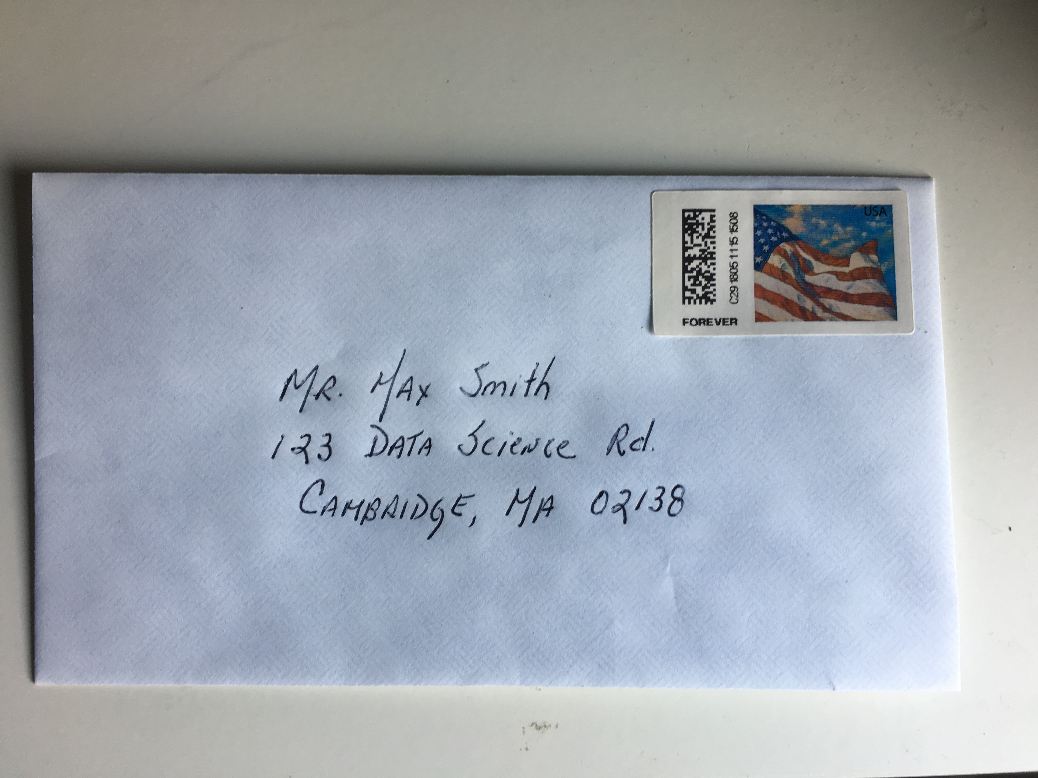
In the Machine Learning part of this book, we will describe how we can build computer algorithms to read handwritten digits, which robots then use to sort the letters. To do this, we first need to collect data, which in this case is a high-dimensional dataset and best stored in a matrix.
The MNIST dataset was generated by digitizing thousands of handwritten digits, already read and annotated by humans1. Below are three images of written digits.
The images are converted into \(28 \times 28 = 784\) pixels and, for each pixel, we obtain a grey scale intensity between 0 (white) and 255 (black). The following plot shows the individual variables for each image:

Each digitized image, indexed by \(i\), is represented by 784 numerical variables corresponding to pixel intensities, along with a categorical outcome, or label, specifying the digit (\(0\)-\(9\)) depicted in the image.
Let’s load the data using the dslabs package:
library(tidyverse)
library(dslabs)
mnist <- read_mnist()
The pixel intensities are saved in a matrix:
class(mnist$train$images)
#> [1] "matrix" "array"
The labels associated with each image are included in a vector:
table(mnist$train$labels)
#>
#>    0    1    2    3    4    5    6    7    8    9
#> 5923 6742 5958 6131 5842 5421 5918 6265 5851 5949
To simplify the code below, we will rename these x and y, respectively:
x <- mnist$train$images
y <- mnist$train$labels
21.3 Matrix Operations in R
Before we define and work through the tasks designed to teach matrix operations, we begin by reviewing some basic matrix functionality in R.
Creating a matrix
Scalars, vectors, and matrices are the basic building blocks of linear algebra. We have already encountered vectors in earlier chapters, and in R, scalars are represented as vectors of length 1. We now extend this understanding to matrices, starting with how to create them in R.
We can create a matrix using the matrix function. The first argument is a vector containing the elements that will fill up the matrix. The second and third arguments determine the number of rows and columns, respectively. So, a typical way to create a matrix is to first obtain a vector of numbers containing the elements of the matrix and feed it to the matrix function. For example, to create a \(100 \times 2\) matrix of normally distributed random variables, we write:
Note that by default, the matrix is filled in column by column:
matrix(1:15, 3, 5)
#>      [,1] [,2] [,3] [,4] [,5]
#> [1,]    1    4    7   10   13
#> [2,]    2    5    8   11   14
#> [3,]    3    6    9   12   15
To fill the matrix row by row, we can use the byrow argument:
matrix(1:15, 3, 5, byrow = TRUE)
#>      [,1] [,2] [,3] [,4] [,5]
#> [1,]    1    2    3    4    5
#> [2,]    6    7    8    9   10
#> [3,]   11   12   13   14   15
The function as.vector converts a matrix back into a vector:
If the product of columns and rows does not match the length of the vector provided in the first argument, matrix recycles values. If the length of the vector is a sub-multiple or multiple of the number of rows, this happens without warning:
matrix(1:3, 3, 5)
#>      [,1] [,2] [,3] [,4] [,5]
#> [1,]    1    1    1    1    1
#> [2,]    2    2    2    2    2
#> [3,]    3    3    3    3    3
The function as.matrix() attempts to coerce its input into a matrix:
df <- data.frame(a = 1:2, b = 3:4, c = 5:6)
as.matrix(df)
#>      a b c
#> [1,] 1 3 5
#> [2,] 2 4 6
Dimensions of a matrix
The dimension of a matrix is an important characteristic needed to ensure that certain linear algebra operations can be performed. The dimension is a two-number summary defined as the number of rows \(\times\) the number of columns.
The nrow function tells us how many rows the matrix has. Here is the number of rows in x, previously defined to store the MNIST training data images:
nrow(x)
#> [1] 60000
The function ncol tells us how many columns:
ncol(x)
#> [1] 784
We learn that our dataset contains 60,000 observations (images) and 784 variables (pixels).
The dim function returns the rows and columns:
dim(x)
#> [1] 60000   784
Now we can confirm that R follows the convention of defining vectors of length \(n\) as \(n\times 1\) matrices or column vectors:
Subsetting
To extract a specific entry from a matrix, for example, the 300th row of the 100th column, we write:
x[300, 100]We can extract subsets of the matrices by using vectors of indices. For example, we can extract the first 100 pixels from the first 300 observations like this:
x[1:300, 1:100]To extract an entire row or subset of rows, we leave the column dimension blank. So the following code returns all the pixels for the first 300 observations:
x[1:300,]Similarly, we can subset any number of columns by keeping the first dimension blank. Here is the code to extract the first 100 pixels:
x[,1:100]The transpose
A common operation when working with matrices is the transpose. We use the transpose to understand several concepts described in the next several sections. This operation simply converts the rows of a matrix into columns. We use the symbols \(\top\) or \('\) next to the bold upper case letter to denote the transpose:
\[ \text{if } \, \mathbf{X} = \begin{bmatrix} x_{11}&\dots & x_{1p} \\ x_{21}&\dots & x_{2p} \\ \vdots & \ddots & \vdots & \\ x_{n1}&\dots & x_{np} \end{bmatrix} \text{ then }\, \mathbf{X}^\top = \begin{bmatrix} x_{11}&x_{21}&\dots & x_{n1} \\ \vdots & \vdots & \ddots & \vdots \\ x_{1p}&x_{2p}&\dots & x_{np} \end{bmatrix} \]
In R, we compute the transpose using the function t
One use of the transpose is that we can write the matrix \(\mathbf{X}\) as rows of the column vectors representing the variables for each individual observation in the following way:
\[ \mathbf{X} = \begin{bmatrix} \mathbf{x}_1^\top\\ \mathbf{x}_2^\top\\ \vdots\\ \mathbf{x}_n^\top \end{bmatrix} \]
Row and column summaries
A common operation with matrices is to apply the same function to each row or to each column. For example, we may want to compute row averages and standard deviations. The apply function lets you do this. The first argument is the matrix, the second is the dimension—1 for rows or 2 for columns—and the third is the function to be applied.
So, for example, to compute the averages and standard deviations of each row, we write:
To compute these for the columns, we simply change the 1 to a 2:
Because these operations are so common, special functions are available to perform them. So, for example, the function rowMeans computes the average of each row:
avg <- rowMeans(x)and the function rowSds from the matrixStats package computes the standard deviations for each row:
library(matrixStats)
sds <- rowSds(x)
The functions colMeans and colSds provide the version for columns.
For other fast implementations of common operations, take a look at what is available in the matrixStats package.
Conditional filtering
One of the advantages of matrix operations over tidyverse operations is that we can easily select columns based on summaries of the columns.
Note that logical filters can be used to subset matrices in a similar way to how they can be used to subset vectors. Here is a simple example subsetting columns with logicals:
This implies that we can select rows with a conditional expression. In the following example, we remove all observations containing at least one NA:
This being a common operation, we have a matrixStats function to do it faster:
x[!rowAnyNAs(x),]Indexing with matrices
An operation that facilitates efficient coding is that we can change entries of a matrix based on conditionals applied to that same matrix. Here is a simple example:
mat <- matrix(1:15, 3, 5)
mat[mat > 6 & mat < 12] <- 0
mat
#>      [,1] [,2] [,3] [,4] [,5]
#> [1,]    1    4    0    0   13
#> [2,]    2    5    0    0   14
#> [3,]    3    6    0   12   15
A useful application of this approach is that we can change all the NA entries of a matrix to something else:
x[is.na(x)] <- 021.4 Vectorization for matrices
Vectorization is one of the main reasons R is so efficient for numerical computation with data. Many operations that would otherwise require explicit loops can instead be applied directly to entire matrices or vectors, making the code both faster and easier to read.
Matrix–vector operations
A common example of matrix vectorization is centering rows: subtracting the mean of each row from its corresponding entries. Although this can be done with the scale() function
scale(x, scale = FALSE)R’s vectorization rules make it possible to achieve this more directly and efficiently. We use row centering as an example, but this approach applies broadly to many operations discussed throughout this chapter.
In R, if we subtract a vector a from a matrix x: x-a, the first element of a is subtracted from the first row, the second element from the second row, and so on. Mathematically, this operation can be written as:
\[ \begin{bmatrix} X_{11}&\dots & X_{1p} \\ X_{21}&\dots & X_{2p} \\ \vdots & \ddots & \vdots \\ X_{n1}&\dots & X_{np} \end{bmatrix} - \begin{bmatrix} a_1\\ a_2\\ \vdots \\ a_n \end{bmatrix} = \begin{bmatrix} X_{11}-a_1&\dots & X_{1p}-a_1\\ X_{21}-a_2&\dots & X_{2p}-a_2\\ \vdots & \ddots & \vdots\\ X_{n1}-a_n&\dots & X_{np}-a_n \end{bmatrix} \]
This means we can center each row of x with this single line of code:
x - rowMeans(x)The same vectorization applies to other arithmetic operations, such as division. For example, we can both center and scale the rows with:
This is equivalent to scale(x), but done explicitly to show the underlying vectorized operations.
The sweep function
If we instead want to scale the columns, the following code will not work as expected because subtraction is applied row-wise:
x - colMeans(x)One workaround is to transpose the matrix, apply the operation, and transpose back:
This works, but it’s cumbersome and inefficient for large matrices due to repeated transpositions.
The sweep function provides a clearer and more general solution for performing vectorized operations on matrices. It is similar to apply, but designed specifically for array-like data and elementwise arithmetic.
When used with a matrix x, sweep takes three main arguments:
-
MARGIN: which dimension to operate over (1for rows,2for columns) -
STATS: the vector of values to sweep out (e.g., means or standard deviations) -
FUN: the operation to apply (default is subtraction"-")
For example, to subtract each column’s mean, we write:
This centers each column so that its average is zero. Because R allows omitting argument names when defaults are clear, a concise and common shorthand is:
Similarly, to center rows we write:
(Though note that x - rowMeans(x) is typically faster for this specific operation.)
To scale rather than center, simply change the operation:
The sweep function also generalizes beyond matrices: it can handle arrays with more than two dimensions and statistics vectors (STATS) of matching dimensions.
Matrix-matrix operations
In R, if you add, subtract, multiply, or divide two matrices, the operation is done element-wise. For example, if two matrices are stored in x and y, then x*y does not result in matrix multiplication as defined in Section 22.1. Instead, the entry in row \(i\) and column \(j\) of this product is the product of the entry in row \(i\) and column \(j\) of x and y, respectively.
21.5 Motivating tasks
To motivate the use of matrices in R, we will pose six tasks that illustrate how matrix operations can help with data exploration of the handwritten digits dataset. Each task highlights a basic matrix operation that is commonly used in R. By seeing how these operations can be implemented with fast and simple code, you will gain hands-on experience with the kinds of computations that arise frequently in high-dimensional data analysis. The primary goal of these tasks is to help you learn how matrix operations work in practice.
Visualize the original image
The pixel intensities are provided as rows in a matrix. Using what we learned in Section 21.3.1, we can convert each row into a \(28 \times 28\) matrix that we can visualize as an image. As an example, we will use the third observation. From the label, we know this is a 4:
y[3]
#> [1] 4
The third row of the matrix x[3,] contains the 784 pixel intensities. If we assume these were entered in order, we can convert them back to a \(28 \times 28\) matrix using:
grid <- matrix(x[3,], 28, 28)To visualize the data, we can use image in the following way:
image(1:28, 1:28, grid)However, because the y-axis in image goes from bottom to top and x stores pixels from top to bottom, the code above shows a flipped image. To flip it back, we can use:
image(1:28, 1:28, grid[, 28:1])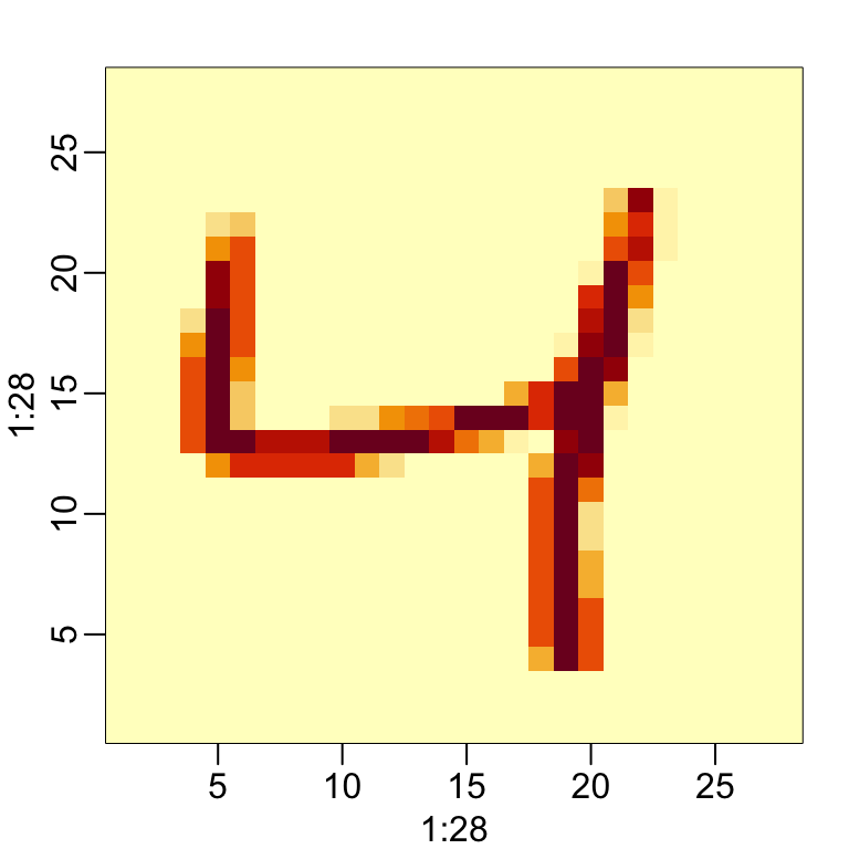
Do some digits require more ink to write than others?
Let’s study the distribution of the total pixel darkness and how it varies by digits.
We can use what we learned in Section 21.3.5 to compute this average for each observation and stratify the values by digit using a boxplot:
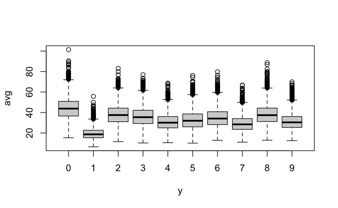
From this plot, we see that, not surprisingly, 1s use less ink than other digits.
Are some pixels uninformative?
We now examine the variation of each pixel across digits to identify and remove those that provide little information for classification. Pixels that show little variation across images do not help distinguish between digits and can safely be excluded. In many cases, removing uninformative features not only simplifies the analysis but also reduces the dataset’s size substantially, improving computational speed.
Using what we learned in Sections 21.3.5 and 21.3.6, we can efficiently compute and filter out such columns. To quantify each pixel’s variability, we calculate its standard deviation across all images using the colSds function from the matrixStats package:
sds <- colSds(x)A quick look at the distribution of these values shows that some pixels have very low entry-to-entry variability:
hist(sds, breaks = 30, main = "SDs")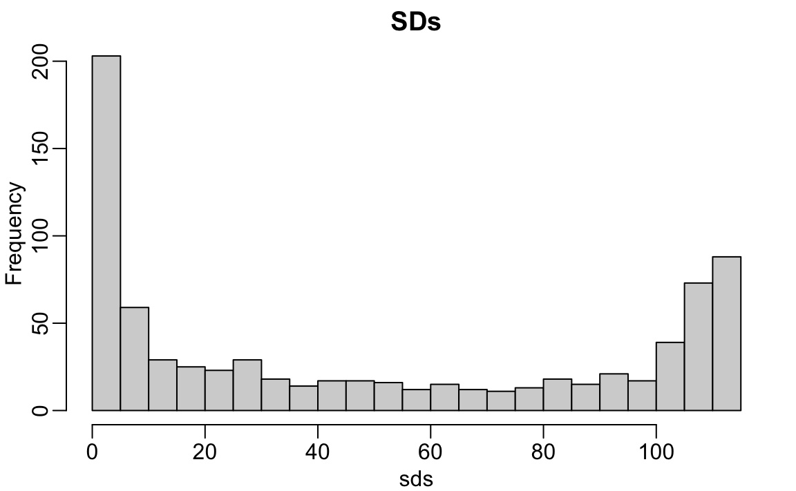
This makes sense since we don’t write in some parts of the box. Here is the variance plotted by location after using what we learned in Section 21.3.1 to create a \(28 \times 28\) matrix:
We see that there is little variation in the corners.
We could remove features that have no variation since these can’t help us predict.
So if we wanted to remove uninformative predictors from our matrix, we could write this one line of code:
Only the columns for which the standard deviation is above 60 are kept, which removes over half the predictors.
Can we remove smudges?
We will first look at the distribution of all pixel values.
This shows a clear dichotomy, which is explained as parts of the image with ink and parts without. If we think that values below, say, 50 are smudges, we can quickly make them zero using what we learned in Section 21.3.7:
new_x <- x
new_x[new_x < 50] <- 0
Binarize the data
The histogram above seems to suggest that this data is mostly binary. A pixel either has ink or does not. Applying what we learned in Section 21.3.7, we can binarize the data using just matrix operations:
bin_x <- x
bin_x[bin_x < 255/2] <- 0
bin_x[bin_x > 255/2] <- 1
We can also convert to a matrix of logicals and then coerce to numbers using what we learned in Section 21.4:
bin_x <- (x > 255/2)*1Standardize the digits
Finally, we will scale each column to have the same average and standard deviation.
Using what we learned in Section 21.4 implies that we can scale each row of a matrix as follows:
And for the columns, we can combine two calls to sweep:
Note that we can use this to standardize rows as well by replacing 2 with 1, and use rowMeans and rowSds.
Finally, note that equivalent functionality can often be achieved with:
This version can be faster for large matrices, though it’s less explicit about what’s happening.
21.6 Exercises
1. Create a 100 by 10 matrix of randomly generated normal numbers. Put the result in x.
2. Apply the three R functions that give you the dimension of x, the number of rows of x, and the number of columns of x, respectively.
3. Add the scalar 1 to row 1, the scalar 2 to row 2, and so on, to the matrix x.
4. Add the scalar 1 to column 1, the scalar 2 to column 2, and so on, to the matrix x. Hint: Use sweep with FUN = "+".
5. Compute the average of each row of x.
6. Compute the average of each column of x.
7. For each digit in the MNIST training data, compute the proportion of pixels that are in a grey area, defined as values between 50 and 205. Make a boxplot by digit class. Hint: Use logical operators and rowMeans.
http://yann.lecun.com/exdb/mnist/↩︎