x_hat <- 0.48
se <- sqrt(x_hat*(1 - x_hat)/25)
se
#> [1] 0.09998 Central Limit Theorem
In Section 5.7 of the Probability part of the book, we introduced the Central Limit Theorem (CLT) as one of the most powerful results in statistics. We learned that, when the sample size is large, the sum or average of independent draws from a population has a distribution that is approximately normal, regardless of the shape of the original population distribution.
In this chapter, we revisit the CLT from an inferential perspective. In probability, we used it to describe the behavior of random variables such as the total winnings in a roulette game. Now, our goal is to use it to quantify the uncertainty in estimates computed from data. In our poll example, the CLT tells us that the sample average \(\bar{X}\) follows an approximately normal distribution centered at the true population parameter, with a standard error that depends on the sample size.
This approximation allows us to answer practical questions such as:
What is the probability that our sample proportion \(\bar{X}\) is within 2% of the true value \(p\)?
In the remainder of this chapter, we will see how the CLT helps answer this question and provides the foundation for confidence intervals, hypothesis testing, and many of the inferential tools used throughout statistics.
8.1 Margin of Error
In practice, pollsters summarize uncertainty using a single, easy-to-interpret number called the margin of error. The margin of error, together with the estimate of the parameter, allows them to report an interval that they are very confident contains the true value. But what does “very confident” actually mean? Using the CLT, we can quantify this statement and connect it directly to probability.
To understand how the margin of error arises, let’s return to the question above and compute:
\[ \Pr(| \bar{X} - p| \leq 0.02) = \Pr(\bar{X} \leq p + 0.02) - \Pr(\bar{X} \leq p - 0.02). \]
We start by standardizing \(\bar{X}\), subtracting its expected value and dividing by its standard error, to obtain a standard normal random variable, denoted by \(Z\):
\[ Z = \frac{\bar{X} - \mathrm{E}[\bar{X}]}{\mathrm{SE}[\bar{X}]}. \]
Since \(p\) is the expected value and \(\mathrm{SE}(\bar{X}) = \sqrt{p(1 - p)/N}\) is the standard error, we can rewrite the probability above as:
\[ \Pr(\bar{X}\leq p + 0.02) - \Pr(\bar{X} \leq p - 0.02) = \Pr\left(Z \leq \frac{0.02}{\mathrm{SE}(\bar{X})} \right) - \Pr\left(Z \leq -\frac{0.02}{\mathrm{SE}(\bar{X})} \right). \]
The challenge is that we do not know \(p\), and therefore we do not know \(\mathrm{SE}(\bar{X})\). However, the CLT still works if we estimate the standard error by substituting \(\bar{X}\) for \(p\). We call this a plug-in estimate:
\[ \hat{\mathrm{SE}}(\bar{X}) = \sqrt{\bar{X}(1 - \bar{X})/N}. \]
In statistics, a hat symbol indicates an estimate obtained from data. Using the observed sample and \(N\), we can compute this estimated standard error.
Let’s continue our calculation using \(\hat{\mathrm{SE}}(\bar{X})\). In our first sample, we had 12 blue and 13 red balls, giving \(\bar{X} = 0.48\). The estimated standard error is:
Now, we can compute the probability that our estimate is within 2% of the true value:
There is only a small chance of being this close to \(p\). A poll of just \(N = 25\) people is therefore not very informative, especially in a close election.
This reasoning naturally leads to the concept of the margin of error. Conventionally, pollsters report an interval that they are 95% confident contains the true parameter. Under the CLT, this 95% probability corresponds to approximately 1.96 standard errors on each side of the estimate. Hence, the margin of error is defined as:
1.96*se
#> [1] 0.196
Why 1.96? Because if we ask for the probability of being within 1.96 standard errors of \(p\), we get:
\[ \Pr(Z \leq 1.96) - \Pr(Z \leq -1.96), \]
which equals about 95%:
Thus, there is a 95% probability that \(\bar{X}\) will fall within \(1.96 \times \hat{\mathrm{SE}}(\bar{X})\) of \(p\). In our case, this corresponds to roughly 0.2. The choice of 95% is somewhat arbitrary, other levels are used in practice, but it is the most common convention. For simplicity, the factor 1.96 is often rounded to 2.
In summary, the CLT tells us that our poll based on \(N = 25\) is not particularly useful: the margin of error is too large to draw meaningful conclusions. We can only say that the race is unlikely to be a landslide. This is why pollsters rely on much larger sample sizes.
From the Real Clear Politics table in the previous chapter, we saw that typical sample sizes range from 700 to 3,500. To see why this matters, consider that if we had obtained \(\bar{X} = 0.48\) with a sample size of 2,000, our estimated standard error would have been 0.0111714. The result would be an estimate of 48% with a margin of error of 2%. This much smaller margin of error would yield a far more informative result—suggesting that red slightly outnumbers blue. Of course, this is hypothetical; we did not conduct a poll of 2,000 to avoid spoiling the competition.
8.2 A Monte Carlo simulation
Suppose we want to use a Monte Carlo simulation to corroborate the tools we have developed using probability theory. The problem is, of course, that we don’t know p. We could construct an urn, similar to the one pictured above, and conduct an analog simulation (without a computer). While time-consuming, we could take 10,000 samples, count the beads, and track the proportions of blue. We can use the function take_poll(n = 1000), instead of drawing from an actual urn, but it would still take time to count the beads and enter the results.
Therefore, one approach we can use to corroborate theoretical results is to pick one or several values of p and run simulations. Let’s set p=0.45 and simulate a poll:
In this particular sample, our estimate is x_hat. We can use that code to do a Monte Carlo simulation:
To review, the theory tells us that \(\bar{X}\) is approximately normally distributed, has expected value \(p=\) 0.45, and standard error \(\sqrt{p(1-p)/N}\) = 0.0157321. The simulation confirms this:
A histogram and qqplot confirm that the normal approximation is also accurate:
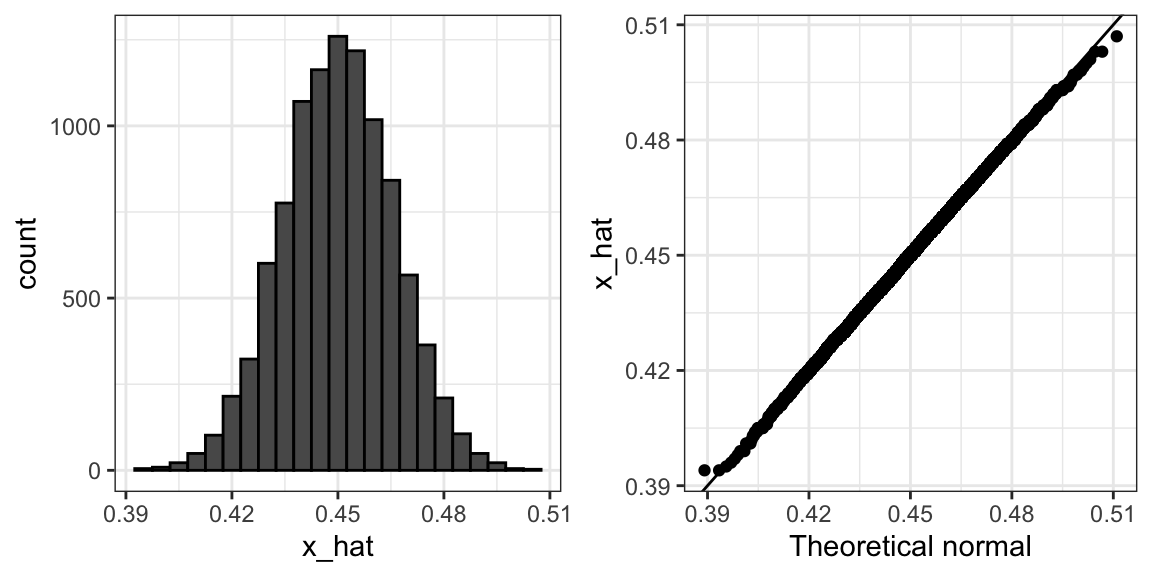
Of course, in real life, we would never be able to run such an experiment because we don’t know \(p\). However, we can run it for various values of \(p\) and \(N\) and see that the theory does indeed work well for most values. You can easily do this by rerunning the code above after changing the values of p and N.
8.3 Bias: Why not run a very large poll?
For realistic values of \(p\), let’s say ranging from 0.35 to 0.65, if we conduct a very large poll with 100,000 people, theory tells us that we would predict the election perfectly, as the largest possible margin of error is around 0.3%:
So why are sample sizes these large not seen? One reason is that conducting such a poll is very expensive. Another, and possibly more important reason, is that theory has its limitations. Polling is much more complicated than simply picking beads from an urn. Some people might lie to pollsters, and others might not have phones. However, perhaps the most important way an actual poll differs from an urn model is that we don’t actually know for sure who is in our population and who is not. How do we know who is going to vote? Are we reaching all possible voters? Hence, even if our margin of error is very small, it might not be exactly right that our expected value is \(p\). We call this bias. Historically, we observe that polls are indeed biased, although not by a substantial amount. The typical bias for the popular vote, for example, appears to be about 2-3%. This makes election forecasting a bit more interesting, and we will explore how to model this in a later section.
8.4 Exercises
1. Write an urn model function that takes the proportion of Democrats \(p\) and the sample size \(N\) as arguments, and returns the sample average if Democrats are 1s and Republicans are 0s. Call the function take_sample.
2. Now assume p <- 0.45 and that your sample size is \(N=100\). Take a sample 10,000 times and save the vector of mean(X) - p into an object called errors. Hint: Use the function you wrote for exercise 1 to write this in one line of code.
3. The vector errors contains, for each simulated sample, the difference between the actual \(p\) and our estimate \(\bar{X}\). We refer to this difference as the error. Compute the average and make a histogram of the errors generated in the Monte Carlo simulation, and select which of the following best describes their distributions:
- The errors are all about 0.05.
- The errors are all about -0.05.
- The errors are symmetrically distributed around 0.
- The errors range from -1 to 1.
4. The error \(\bar{X}-p\) is a random variable. In practice, the error is not observed because we do not know \(p\). Here, we observe it since we constructed the simulation. What is the average size of the error if we define the size by taking the absolute value \(\mid \bar{X} - p \mid\)?
5. The standard error is related to the typical size of the error we make when predicting. For mathematical reasons related to the Central Limit Theorem, we actually use the standard deviation of errors, rather than the average of the absolute values, to quantify the typical size. What is this standard deviation of the errors?
6. The theory we just learned tells us what this standard deviation is going to be because it is the standard error of \(\bar{X}\). What does theory tell us is the standard error of \(\bar{X}\) for a sample size of 100?
7. In practice, we don’t know \(p\), so we construct an estimate of the theoretical prediction by plugging in \(\bar{X}\) for \(p\). Compute this estimate. Set the seed at 1 with set.seed(1).
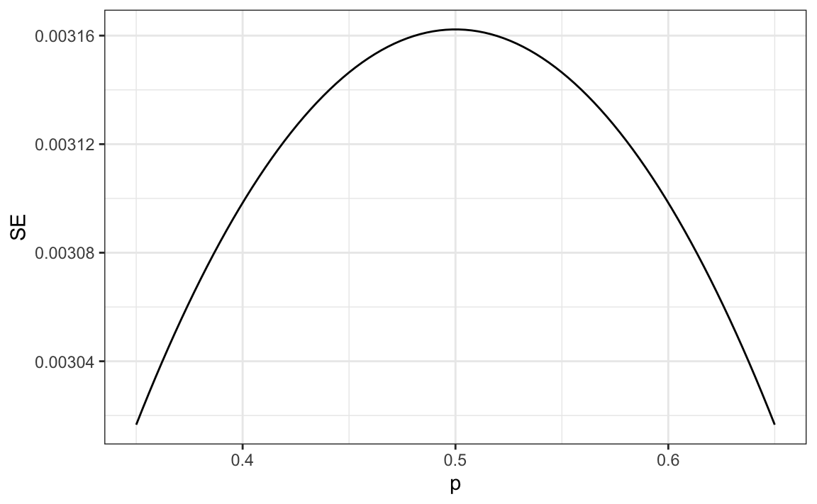
8. Note how close the standard error estimates obtained from the Monte Carlo simulation (exercise 5), the theoretical prediction (exercise 6), and the estimate of the theoretical prediction (exercise 7) are. The theory is working and it gives us a practical approach to knowing the typical error we will make if we predict \(p\) with \(\bar{X}\). Another advantage that the theoretical result provides is that it gives an idea of how large a sample size is required to obtain the precision we need. Earlier, we learned that the largest standard errors occur for \(p=0.5\). Create a plot of the largest standard error for \(N\) ranging from 100 to 5,000. Based on this plot, how large does the sample size have to be to have a standard error of about 1%?
- 100
- 500
- 2,500
- 4,000
9. For sample size \(N=100\), the Central Limit Theorem tells us that the distribution of \(\bar{X}\) is:
- practically equal to \(p\).
- approximately normal with expected value \(p\) and standard error \(\sqrt{p(1-p)/N}\).
- approximately normal with expected value \(\bar{X}\) and standard error \(\sqrt{\bar{X}(1-\bar{X})/N}\).
- not a random variable.
10. Based on the answer from exercise 8, the error \(\bar{X} - p\) is:
- practically equal to 0.
- approximately normal with expected value \(0\) and standard error \(\sqrt{p(1-p)/N}\).
- approximately normal with expected value \(p\) and standard error \(\sqrt{p(1-p)/N}\).
- not a random variable.
11. To corroborate your answer to exercise 9, make a qq-plot of the errors you generated in exercise 2 to see if they follow a normal distribution.
12. If \(p=0.45\) and \(N=100\) as in exercise 2, use the CLT to estimate the probability that \(\bar{X}>0.5\). Assume you know \(p=0.45\) for this calculation.
13. Assume you are in a practical situation and you don’t know \(p\). Take a sample of size \(N=100\) and obtain a sample average of \(\bar{X} = 0.51\). What is the CLT approximation for the probability that your error is equal to or larger than 0.01?